Finite elements in 2D and 3D

Finite element approximation is particularly powerful in 2D and 3D because the method can handle a geometrically complex domain \(\Omega\) with ease. The principal idea is, as in 1D, to divide the domain into cells and use polynomials for approximating a function over a cell. Two popular cell shapes are triangles and the quadrilaterals. Figures Examples on 2D P1 elements, Examples on 2D P1 elements in a deformed geometry, and Examples on 2D Q1 elements provide examples. P1 elements means linear functions (\(a_0 + a_1x + a_2y\)) over triangles, while Q1 elements have bilinear functions (\(a_0 + a_1x + a_2y + a_3xy\)) over rectangular cells. Higher-order elements can easily be defined.

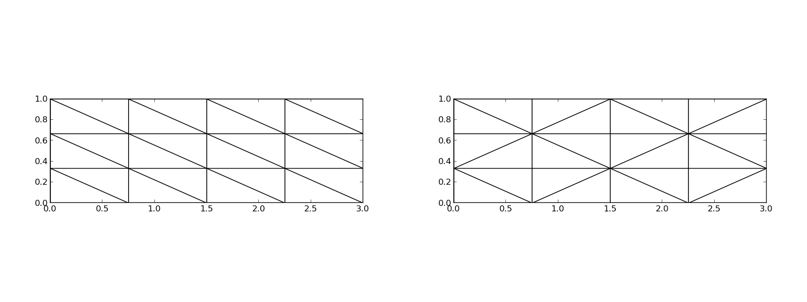
Examples on 2D P1 elements

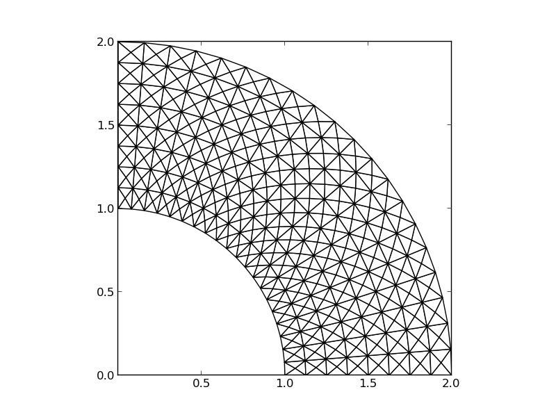
Examples on 2D P1 elements in a deformed geometry

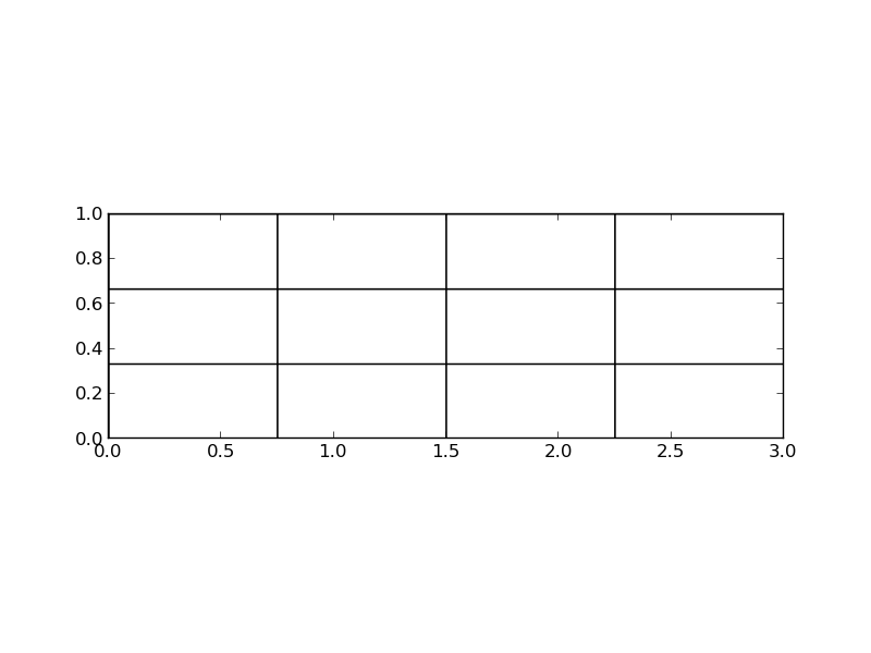
Examples on 2D Q1 elements

Basis functions over triangles in the physical domain

Cells with triangular shape will be in main focus here. With the P1 triangular element, \(u\) is a linear function over each cell, as depicted in Figure Example on piecewise linear 2D functions defined on triangles, with discontinuous derivatives at the cell boundaries.

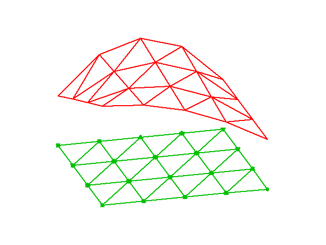
Example on piecewise linear 2D functions defined on triangles

We give the vertices of the cells global and local numbers as in 1D. The degrees of freedom in the P1 element are the function values at a set of nodes, which are the three vertices. The basis function \({\varphi}_i(x,y)\) is then 1 at the vertex with global vertex number \(i\) and zero at all other vertices. On an element, the three degrees of freedom uniquely determine the linear basis functions in that element, as usual. The global \({\varphi}_i(x,y)\) function is then a combination of the linear functions (planar surfaces) over all the neighboring cells that have vertex number \(i\) in common. Figure Example on a piecewise linear 2D basis function over a patch of triangles tries to illustrate the shape of such a “pyramid”-like function.

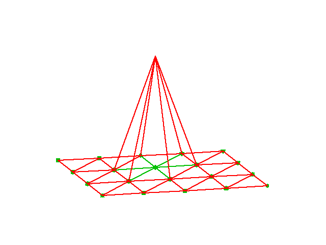
Example on a piecewise linear 2D basis function over a patch of triangles

Element matrices and vectors

As in 1D, we split the integral over \(\Omega\) into a sum of integrals over cells. Also as in 1D, \({\varphi}_i\) overlaps \({\varphi}_j\) (i.e., \({\varphi}_i{\varphi}_j\neq 0\)) if and only if \(i\) and \(j\) are vertices in the same cell. Therefore, the integral of \({\varphi}_i{\varphi}_j\) over an element is nonzero only when \(i\) and \(j\) run over the vertex numbers in the element. These nonzero contributions to the coefficient matrix are, as in 1D, collected in an element matrix. The size of the element matrix becomes \(3\times 3\) since there are three degrees of freedom that \(i\) and \(j\) run over. Again, as in 1D, we number the local vertices in a cell, starting at 0, and add the entries in the element matrix into the global system matrix, exactly as in 1D. All details and code appear below.

Basis functions over triangles in the reference cell

As in 1D, we can define the basis functions and the degrees of freedom in a reference cell and then use a mapping from the reference coordinate system to the physical coordinate system. We also have a mapping of local degrees of freedom numbers to global degrees of freedom numbers.

The reference cell in an \((X,Y)\) coordinate system has vertices \((0,0)\), \((1,0)\), and \((0,1)\), corresponding to local vertex numbers 0, 1, and 2, respectively. The P1 element has linear functions \({\tilde{\varphi}}_r(X,Y)\) as basis functions, \(r=0,1,2\). Since a linear function \({\tilde{\varphi}}_r(X,Y)\) in 2D is on the form \(C_{r,0} + C_{r,1}X + C_{r,2}Y\), and hence has three parameters \(C_{r,0}\), \(C_{r,1}\), and \(C_{r,2}\), we need three degrees of freedom. These are in general taken as the function values at a set of nodes. For the P1 element the set of nodes is the three vertices. Figure 2D P1 element displays the geometry of the element and the location of the nodes.

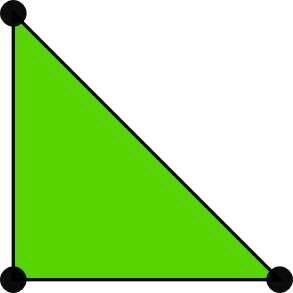
2D P1 element

Requiring \({\tilde{\varphi}}_r=1\) at node number \(r\) and \({\tilde{\varphi}}_r=0\) at the two other nodes, gives three linear equations to determine \(C_{r,0}\), \(C_{r,1}\), and \(C_{r,2}\). The result is

\[{\tilde{\varphi}}_0(X,Y) = 1 - X - Y,\]

\[{\tilde{\varphi}}_1(X,Y) = X,\]

\[{\tilde{\varphi}}_2(X,Y) = Y\]

Higher-order approximations are obtained by increasing the polynomial order, adding additional nodes, and letting the degrees of freedom be function values at the nodes. Figure 2D P2 element shows the location of the six nodes in the P2 element.

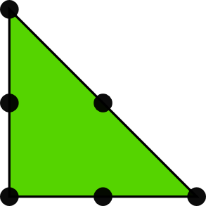
2D P2 element

A polynomial of degree \(p\) in \(X\) and \(Y\) has \(n_p=(p+1)(p+2)/2\) terms and hence needs \(n_p\) nodes. The values at the nodes constitute \(n_p\) degrees of freedom. The location of the nodes for \({\tilde{\varphi}}_r\) up to degree 6 is displayed in Figure 2D P1, P2, P3, P4, P5, and P6 elements.

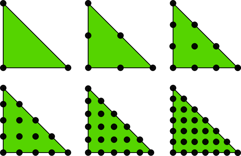
2D P1, P2, P3, P4, P5, and P6 elements

The generalization to 3D is straightforward: the reference element is a tetrahedron with vertices \((0,0,0)\), \((1,0,0)\), \((0,1,0)\), and \((0,0,1)\) in a \(X,Y,Z\) reference coordinate system. The P1 element has its degrees of freedom as four nodes, which are the four vertices, see Figure P1 elements in 1D, 2D, and 3D. The P2 element adds additional nodes along the edges of the cell, yielding a total of 10 nodes and degrees of freedom, see Figure P2 elements in 1D, 2D, and 3D.

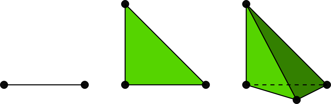
P1 elements in 1D, 2D, and 3D

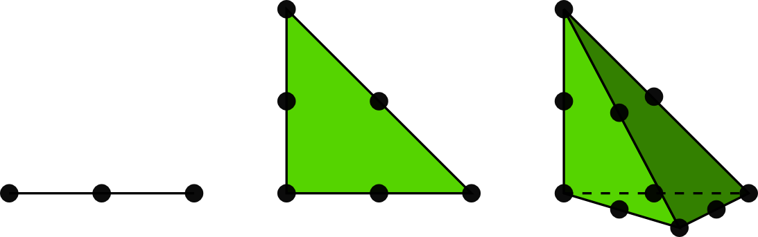
P2 elements in 1D, 2D, and 3D

The interval in 1D, the triangle in 2D, the tetrahedron in 3D, and its generalizations to higher space dimensions are known as simplex cells (the geometry) or simplex elements (the geometry, basis functions, degrees of freedom, etc.). The plural forms simplices and simplexes are also a much used shorter terms when referring to this type of cells or elements. The side of a simplex is called a face, while the tetrahedron also has edges.

Acknowledgment. Figures 2D P1 element to P2 elements in 1D, 2D, and 3D are created by Anders Logg and taken from the FEniCS book: Automated Solution of Differential Equations by the Finite Element Method, edited by A. Logg, K.-A. Mardal, and G. N. Wells, published by Springer, 2012.

Affine mapping of the reference cell

Let \({\tilde{\varphi}}_r^{(1)}\) denote the basis functions associated with the P1 element in 1D, 2D, or 3D, and let \(\boldsymbol{x}_{q(e,r)}\) be the physical coordinates of local vertex number \(r\) in cell \(e\). Furthermore, let \(\boldsymbol{X}\) be a point in the reference coordinate system corresponding to the point \(\boldsymbol{x}\) in the physical coordinate system. The affine mapping of any \(\boldsymbol{X}\) onto \(\boldsymbol{x}\) is then defined by

(1)\[ \boldsymbol{x} = \sum_{r} {\tilde{\varphi}}_r^{(1)}(\boldsymbol{X})\boldsymbol{x}_{q(e,r)},\]

where \(r\) runs over the local vertex numbers in the cell. The affine mapping essentially stretches, translates, and rotates the triangle. Straight or planar faces of the reference cell are therefore mapped onto straight or planar faces in the physical coordinate system. The mapping can be used for both P1 and higher-order elements, but note that the mapping itself always applies the P1 basis functions.

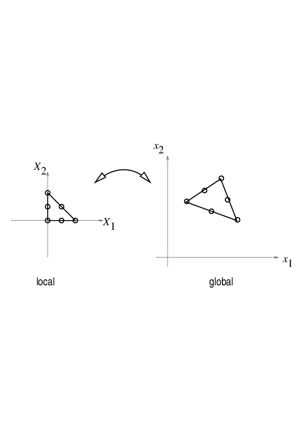
Affine mapping of a P1 element

Isoparametric mapping of the reference cell

Instead of using the P1 basis functions in the mapping (1), we may use the basis functions of the actual Pd element:

(2)\[ \boldsymbol{x} = \sum_{r} {\tilde{\varphi}}_r(\boldsymbol{X})\boldsymbol{x}_{q(e,r)},\]

where \(r\) runs over all nodes, i.e., all points associated with the degrees of freedom. This is called an isoparametric mapping. For P1 elements it is identical to the affine mapping (1), but for higher-order elements the mapping of the straight or planar faces of the reference cell will result in a curved face in the physical coordinate system. For example, when we use the basis functions of the triangular P2 element in 2D in (2), the straight faces of the reference triangle are mapped onto curved faces of parabolic shape in the physical coordinate system, see Figure Isoparametric mapping of a P2 element.

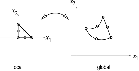
Isoparametric mapping of a P2 element

From (1) or (2) it is easy to realize that the vertices are correctly mapped. Consider a vertex with local number \(s\). Then \({\tilde{\varphi}}_s=1\) at this vertex and zero at the others. This means that only one term in the sum is nonzero and \(\boldsymbol{x}=\boldsymbol{x}_{q(e,s)}\), which is the coordinate of this vertex in the global coordinate system.

Computing integrals

Let \(\tilde\Omega^r\) denote the reference cell and \(\Omega^{(e)}\) the cell in the physical coordinate system. The transformation of the integral from the physical to the reference coordinate system reads

\[\int_{\Omega^{(e)}}{\varphi}_i (\boldsymbol{x}) {\varphi}_j (\boldsymbol{x}) {\, \mathrm{d}x} = \int_{\tilde\Omega^r} {\tilde{\varphi}}_i (\boldsymbol{X}) {\tilde{\varphi}}_j (\boldsymbol{X}) \det J\, {\, \mathrm{d}X},\]

\[\int_{\Omega^{(e)}}{\varphi}_i (\boldsymbol{x}) f(\boldsymbol{x}) {\, \mathrm{d}x} = \int_{\tilde\Omega^r} {\tilde{\varphi}}_i (\boldsymbol{X}) f(\boldsymbol{x}(\boldsymbol{X})) \det J\, {\, \mathrm{d}X},\]

where \({\, \mathrm{d}x}\) means the infinitesimal area element \(dx dy\) in 2D and \(dx dy dz\) in 3D, with a similar definition of \({\, \mathrm{d}X}\). The quantity \(\det J\) is the determinant of the Jacobian of the mapping \(\boldsymbol{x}(\boldsymbol{X})\). In 2D,

(3)\[\begin{split} J = \left[\begin{array}{cc} \frac{\partial x}{\partial X} & \frac{\partial x}{\partial Y}\\ \frac{\partial y}{\partial X} & \frac{\partial y}{\partial Y} \end{array}\right], \quad \det J = \frac{\partial x}{\partial X}\frac{\partial y}{\partial Y} - \frac{\partial x}{\partial Y}\frac{\partial y}{\partial X} {\thinspace .}\end{split}\]

With the affine mapping (1), \(\det J=2\Delta\), where \(\Delta\) is the area or volume of the cell in the physical coordinate system.

Remark. Observe that finite elements in 2D and 3D builds on the same ideas and concepts as in 1D, but there is simply much more to compute because the specific mathematical formulas in 2D and 3D are more complicated and the book keeping with dof maps also gets more complicated. The manual work is tedious, lengthy, and error-prone so automation by the computer is a must.