Advanced partial differential equation models
This final chapter addresses more complicated PDE models, including linear elasticity, viscous flow, heat transfer, porous media flow, gas dynamics, and electrophysiology. A range of classical dimensionless numbers are discussed in terms of the scaling.
The equations of linear elasticity
To the best of the authors’ knowledge, it seems that mathematical models in elasticity and structural analysis are almost never non-dimensionalized. This is probably due to tradition, but the following sections will demonstrate the usefulness of scaling also in this scientific field.
We start out with the general, time-dependent elasticity PDE with variable material properties. Analysis based on scaling is used to determine under what circumstances the acceleration term can be neglected and we end up with the widely used stationary elasticity PDE. Scaling of different types of boundary conditions is also treated. At the end, we scale the equations of coupled thermo-elasticity. All the models make the assumption of small displacement gradients and Hooke’s generalized constitutive law such that linear elasticity theory applies.
The general time-dependent elasticity problem
The following vector PDE governs deformation and stress in purely elastic materials, under the assumption of small displacement gradients:
Here, \(\boldsymbol{u}\) is the displacement vector, \(\varrho\) is the density of the material, \(\lambda\) and \(\mu\) are the Lame elasticity parameters, and \(\boldsymbol{f}\) is a body force (gravity, centrifugal force, or similar).
We introduce dimensionless variables:
Also the elasticity parameters and the density can be scaled, if they are not constants,
where the characteristic quantities are typically spatial maximum values of the functions:
Finally, we scale \(\boldsymbol{f}\) too (if not constant):
Inserting the dimensionless quantities in the governing vector PDE results in
Making the terms non-dimensional gives the equation
We may choose \(t_c\) to make the coefficient in front of any of the spatial derivative terms equal unity. Here we choose the \(\mu\) term, which implies
The scale for \(\boldsymbol{u}\) can be chosen from an initial displacement or by making the coefficient in front of the \(\bar{\boldsymbol{f}}\) term unity. The latter means
As discussed later, in the section The stationary elasticity problem, this might not be the desired \(u_c\) in applications.
The resulting dimensionless PDE becomes
The only dimensionless parameter is
If the source term is absent, we must use the initial condition or a known boundary displacement to determine \(u_c\).
Dimensionless stress tensor
The stress tensor \(\boldsymbol{\sigma}\) is a key quantity in elasticity and is given by
This \(\boldsymbol{\sigma}\) can be computed as soon as the PDE problem for \(\boldsymbol{u}\) has been solved. Inserting dimensionless variables on the right-hand side of the above relation gives
The coefficient on the right-hand side, \(\mu_c u_cL^{-1}\), has dimension of stress, since (according to the second table in the section Dimensions of common physical quantities) \([\hbox{M}\hbox{T}^{-2}\hbox{L}^{-1})(\hbox{L})(\hbox{L}^{-1})] =[\hbox{M}\hbox{T}^{-2}\hbox{L}^{-1}]\), which is the dimension of stress. The quantity \(\mu_c u_cL^{-1}\) is therefore the natural scale of the stress tensor:
and we have the dimensionless stress-displacement relation
When can the acceleration term be neglected?
A lot of applications of the elasticity equation involve static or quasi-static deformations where the acceleration term \(\varrho\boldsymbol{u}_{tt}\) is neglected. Now we shall see under which conditions the quasi-static approximation holds.
The further discussion will need to look into the time scales of elastic waves, because it turns out that the chosen \(t_c\) above is closely linked to the propagation speed of elastic waves in a homogeneous body without body forces. A relevant model for such waves has constant \(\varrho\), \(\lambda\), and \(\mu\), and no force term:
S waves
Let us take the curl of this PDE and notice that the curl of a gradient vanishes. The result is
i.e., a wave equation for \(\nabla\times\boldsymbol{u}\). The wave velocity is
The corresponding waves are called S waves. The curl of a displacement field is closely related to rotation of continuum elements. S waves are therefore rotation waves, also sometimes referred to as shear waves.
The divergence of a displacement field can be interpreted as the volume change of continuum elements. Suppose this volume change vanishes, \(\nabla\cdot\boldsymbol{u} = 0\), which means that the material is incompressible. The elasticity equation then simplifies to
so each component of the displacement field in this case also propagates as a wave with speed \(c_S^2\). The time it takes for such a wave to travel one characteristic length \(L\) is \(L/c_S\), i.e., \(L\sqrt{\varrho/\mu}\), which is nothing but our characteristic time \(t_c\).
P waves
We may take the divergence of the PDE instead and notice that \(\nabla\cdot\nabla =\nabla^2\) so
with wave velocity
That is, the volume change (expansion/compression) propagates as a wave with speed \(c_P\). These types of waves are called P waves. Other names are pressure and expansion/compression waves.
Suppose now that \(\nabla\times\boldsymbol{u} =0\), i.e., there is no rotation (“shear”) of continuum elements. Mathematically this condition implies that \(\nabla^2\boldsymbol{u} = \nabla(\nabla\cdot\boldsymbol{u})\) (see any book on vector calculus or Wikipedia). Our model equation (204) then reduces to
which is nothing but a wave equation for the expansion component of the displacement field, just as (205) is for the shear component.
Time-varying load
Suppose we have some time-varying boundary condition on \(\boldsymbol{u}\) or the stress vector (traction), with a time scale \(1/\omega\) (some oscillating movement that goes like \(\sin\omega t\), for instance). We choose \(t_c=1/\omega\). The scaling now leads to
where we have set
as before, and \(\gamma\) is a new dimensionless number,
The last rewrite shows that \(\sqrt{\gamma}\) is the ratio of the time scale for S waves and the time scale for the forced movement on the boundary. The acceleration term can therefore be neglected when \(\gamma\ll 1\), i.e., when the time scale for movement on the boundary is much larger than the time it takes for the S waves to travel through the domain. Since the velocity of S waves in solids is very large and the time scale correspondingly small, \(\gamma\ll 1\) is very often the case in applications involving structural analysis. Exercise 4.1: Comparison of vibration models for elastic structures explores related models and asks for comparisons of time scales for waves and mechanical vibrations in structures.
The stationary elasticity problem
Scaling of the PDE
We now look at the stationary version of (200) where the \(\varrho\boldsymbol{u}_{tt}\) term is removed. The first step in the scaling is just inserting the dimensionless variables:
Dividing by \(L^2u_c\mu_c\) gives
Choosing \(u_c = \varrho L^2f_c/\mu_c\) leads to
A homogeneous material with constant \(\lambda\), \(\mu\), and \(\varrho\) is an interesting case (this corresponds to \(\mu_c=\mu\), \(\lambda_c=\lambda\), \(\varrho_c=\varrho\), \(\bar\varrho=\bar\lambda=\bar\mu=1\)):
Now \(\beta\) is defined as
It shows that in standard, stationary elasticity, \(\lambda/\mu\) is the only significant physical parameter.
Remark on the characteristic displacement
The presented scaling may not be valid for problems where the geometry involves some dimensions that are much smaller than others, such as for beams, shells, or plates. Then one more length scale must be defined which gives us non-dimensional geometrical numbers. Global balances of moments and loads then determine how characteristic displacements depend on these numbers. As an example, consider a cantilever beam of length \(L\) and square-shaped cross section of width \(W\), deformed under its own weight. From beam theory one can derive \(u_c = \frac{3}{2}\varrho g L^2\delta^2/E\), where \(\delta = L/W\) (\(g\) is the acceleration of gravity). If we consider \(E\) to be of the same size as \(\lambda\), this implies that \(\gamma\sim\delta^{-2}\). So, it may be wise to prescribe a \(u_c\) in elasticity problems, perhaps from formulas as shown, and keep \(\gamma\) in the PDE.
Scaling of displacement boundary conditions
A typical boundary condition on some part of the boundary is a prescribed displacement. For simplicity, we set \(\boldsymbol{u} = \boldsymbol{U}_0\) for a constant vector \(\boldsymbol{U}_0\) as boundary condition. With \(u_c=\varrho L^2f_c/\mu\), we get the dimensionless condition
In the absence of body forces, the expression for \(u_c\) has no meaning (\(f_c=0\)), so then \(u_c = |\boldsymbol{U}_0|\) is a better choice. This gives the dimensionless boundary condition
which is the unit vector in the direction of \(\boldsymbol{U}_0\). The new \(u_c\) changes the coefficient in front of the body force term, if that term is present, to the dimensionless number
Scaling of traction boundary conditions
The other type of common boundary condition in elasticity is a prescribed traction (stress vector) on some part of the boundary:
where, to make it simple, we take \(\boldsymbol{T}_0\) as a constant vector. From the section Dimensionless stress tensor we have a stress scale \(\sigma_c = \mu u_c/L\), but we may alternatively use \(|\boldsymbol{T}_0|\) as stress scale. In that case,
which is a unit vector in the direction of \(\boldsymbol{T}_0\). Many applications involve large traction free areas on the boundary, on which we simply have \(\bar{\boldsymbol{\sigma}}\cdot\boldsymbol{n} = 0\).
Quasi-static thermo-elasticity
Heating solids gives rise to expansion, i.e., strains, which may cause stress if displacements are constrained. The time scale of temperature changes are usually much larger than the time scales of elastic waves, so the stationary equations of elasticity can be used, but a term depends on the temperature, so the equations must be coupled to a PDE for heat transfer in solids. The resulting system of PDEs is known as the equations of thermo-elasticity and reads
where \(T\) is the temperature, \(\alpha\) is a coefficient of thermal expansion, \(c\) is a heat capacity, \(\kappa\) is the heat conduction coefficient, and \(\boldsymbol{f}_T\) is some heat source. The density \(\varrho\) is strictly speaking a function of \(T\) and the stress state, but a widely used approximation is to consider \(\varrho\) as a constant. Most thermo-elasticity applications have \(\boldsymbol{f}_T=0\), so we drop this term. Most applications also involve some heating from a temperature level \(T_0\) to some level \(T_0 +\Delta T\). A suitable scaling for \(T\) is therefore
so that \(\bar{T}\in [0,1]\). The elasticity equation has already been scaled and so has the diffusion equation for \(T\). We base the time scale on the diffusion, i.e., the thermal conduction process:
We imagine that \(\kappa\) is scaled as \(\bar\kappa = \kappa/\kappa_c\). The dimensionless PDE system then becomes
Here we have chosen \(u_c\) such that the “heating source term” has a unit coefficient, acknowledging that this thermal expansion balances the stress terms with \(\bar{\boldsymbol{u}}\). The corresponding displacement scale is
The dimensionless number in the body force term is therefore
which measures the ratio of the body force term and the “heating source term”.
A homogeneous body with constant \(\varrho\), \(\lambda\), \(\mu\), \(c\), and \(\kappa\) is common. The PDE system reduces in this case to
In the absence of body forces, \(\beta\) is again the key parameter.
The boundary conditions for thermo-elasticity consist of the conditions for elasticity and the conditions for diffusion. Scaling of such conditions are discussed in the section The diffusion equation and The stationary elasticity problem.
The Navier-Stokes equations
This section shows how to scale various versions of the equations governing incompressible viscous fluid flow. We start with the plain Navier-Stokes equations without body forces and progress with adding the gravity force and a free surface. We also look at scaling low Reynolds number flow and oscillating flows.
The momentum equation without body forces
The Navier-Stokes equations for incompressible viscous fluid flow, without body forces, take the form
The primary unknowns are the velocity \(\boldsymbol{u}\) and the pressure \(p\). Moreover, \(\varrho\) is the fluid density, and \(\mu\) is the dynamic viscosity.
Scaling
We start, as usual, by introducing a notation for dimensionless independent and dependent variables:
where \(L\) is some characteristic distance, \(t_c\) is some characteristic time, \(u_c\) is a characteristic velocity, while \(p_c\) is a characteristic pressure. Inserted in the equations,
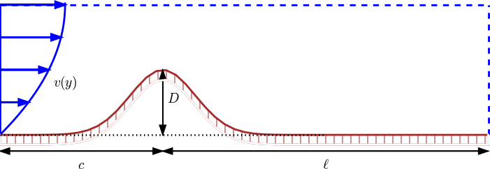
For the velocity it is common to just introduce some \(U\) for \(u_c\). This \(U\) is normally implied by the problem description. For example, in the flow configuration below, with flow over a bump, we have some incoming flow with a profile \(v(y)\) and \(U\) can typically be chosen as \(U=\max_y v(y)\). The height of the bump influences the wake behind the bump, and is the length scale that really impacts the flow, so it is natural to set \(L=D\). For numerical simulations in a domain of finite extent, \([0,c+\ell]\), \(c\) must be large enough to avoid feedback on the inlet profile, and \(\ell\) must be large enough for the type of outflow boundary condition used. Ideally, \(c,\ell\rightarrow\infty\), so none of these parameters are useful as length scales.
For flow in a channel or tube, we also have some inlet profile, e.g., \(v(r)\) in a tube, where \(r\) is the radial coordinate. A natural choice of characteristic velocity is \(U=v(0)\) or to let \(U\) be the average flow, i.e.,
if \(R\) is the radius of the tube. Other examples may be flow around a body, where there is some distant constant inlet flow \(\boldsymbol{u} = U_0\boldsymbol{i}\), for instance, and \(U=U_0\) is an obvious choice. We therefore assume that the flow problem itself brings a natural candidate for \(U\).
Having a characteristic distance \(L\) and velocity \(U\), an obvious time measure is \(L/U\) so we set \(t_c=L/U\). Dividing by the coefficient in front of the time derivative term, creates a pressure term
The coefficient suggest a choice \(p_c=\varrho U^2\) if the pressure gradient term is to have the same size as the acceleration terms. This \(p_c\) is a very common pressure scale in fluid mechanics, arising from Bernoulli’s equation
for stationary flow.
Dimensonless PDEs and the Reynolds number
The discussions so far result in the following dimensionless form of (215) and (216):
where Re is the famous Reynolds number,
The latter expression makes use of the kinematic viscosity \(\nu = \mu/\varrho\). For viscous fluid flows without body forces there is hence only one dimensionless number, Re.
The Reynolds number can be interpreted as the ratio of convection and viscosity:
(We have here used that \(\nabla\boldsymbol{u}\) goes like \(U/L\) and \(\nabla^2\boldsymbol{u}\) goes like \(U/L^2\).)
Scaling of time for low Reynolds numbers
As we discussed in the section The convection-diffusion equation for the convection-diffusion equation, there is not just one scaling that fits all problems. Above, we used \(t_c=L/U\), which is appropriate if convection is a dominating physical effect. In case the convection term \(\varrho\boldsymbol{u}\cdot\nabla\boldsymbol{u}\) is much smaller than the viscosity term \(\mu\nabla^2\boldsymbol{u}\), i.e., the Reynolds number is small, the viscosity term is dominating. However, if the scaling is right, the other terms are of order unity, and \(\hbox{Re}^{-1}\nabla^2\bar{\boldsymbol{u}}\) must then also be of unit size. This fact implies that \(\nabla^2\bar{\boldsymbol{u}}\) must be small, but then the scaling is not right (since a right scaling will lead to \(\bar u\) and its derivatives around unity). Such reasoning around inconsistent size of terms clearly points to the need for other scales.
In the low-Reynolds number regime, the diffusion effect of \(\nabla^2\bar{\boldsymbol{u}}\) is dominating, and we should use a time scale based on diffusion rather than convection. Such a time scale is \(t_c = L^2/(\mu/\varrho) = L^2/\nu\). With this time scale, the dimensionless Navier-Stokes equations look like
As stated in the box in the section The convection-diffusion equation, (221) is the appropriate PDE for very low Reynolds number flow and suggests neglecting the convection term. If the flow is also steady, the time derivative term can be neglected, and we end up with the so-called Stokes problem for steady, slow, viscous flow:
This flow regime is also known as Stokes’ flow or creeping flow.
Shear stress as pressure scale
Instead of using the kinetic energy \(\varrho U^2\) as pressure scale, one can use the shear stress \(\mu U/L\) (\(U/L\) reflects the spatial derivative of the velocity, which enters the shear stress expression \(\mu\partial u/\partial y\)). Using \(U\) as velocity scale, \(L/U\) as time scale, and \(\mu U/L\) as pressure scale, results in
Low Reynolds number flow now suggests neglecting both acceleration terms.
Gravity force and the Froude number
We now add a gravity force to the momentum equation (215):
where \(g\) is the acceleration of gravity, and \(\boldsymbol{k}\) is a unit vector in the opposite direction of gravity. The new term takes the following form after non-dimensionalization:
where Fr is the dimensionless Froude number,
This quantity reflects the ratio of inertia and gravity forces:
Oscillating boundary conditions and the Strouhal number
Many flows have an oscillating nature, often arising from some oscillating boundary condition. Suppose such a condition, at some boundary \(x=\hbox{const}\), takes the specific form
The dimensionless counterpart becomes
if \(t_c=L/U\) is the appropriate time scale. This condition can be written
where St is the Strouhal number,
The two important dimensionless parameters in oscillating flows are then the Reynolds and Strouhal numbers.
Even if the boundary conditions are of steady type, as for flow around a sphere or cylinder, the flow may at certain Reynolds numbers get unsteady and oscillating. For \(10^2 < \hbox{Re} < 10^7\), steady inflow towards a cylinder will cause vortex shedding: an array of vortices are periodically shedded from the cylinder, producing an oscillating flow pattern and force on the cylinder. The Strouhal number is used to characterize the frequency of oscillations. The phenomenon, known as von Karman vortex street, is particularly important if the frequency of the force on the cylinder hits the free vibration frequency of the cylinder such that resonance occurs. The result can be large displacements of the cylinder and structural failure. A famous case in engineering is the failure of the Tacoma Narrows suspension bridge in 1940, when wind-induced vortex shedding caused resonance with the free torsional vibrations of the bridge.
Cavitation and the Euler number
The dimensionless pressure in (219) made use of the pressure scale \(p_c=\varrho U^2\). This is an appropriate scale if the pressure level is not of importance, which is very often the case since only the pressure gradient enters the flow equation and drives the flow. However, there are circumstances where the pressure level is of importance. For example, in some flows the pressure may become so low that the vapor pressure of the liquid is reached and that vapor cavities form (a phenomenon known as cavitation). A more appropriate pressure scale is then \(p_c = p_{\infty} - p_v\), where \(p_\infty\) is a characteristic pressure level far from vapor cavities and \(p_v\) is the vapor pressure. The coefficient in front of the dimensionless pressure gradient is then
Inspired by Bernoulli’s equation \(p + \frac{1}{2}\varrho \boldsymbol{u}\cdot\boldsymbol{u} = \hbox{const}\) in fluid mechanics, a factor \(\frac{1}{2}\) is often inserted in the denominator. The corresponding dimensionless number,
is called the Euler number. The pressure gradient term now reads \(\frac{1}{2}\hbox{Eu}\,\bar\nabla\bar p\). The Euler number expresses the ratio of pressure differences and the kinetic energy of the flow.
Free surface conditions and the Weber number
At a free surface, \(z=\eta(x,y,t)\), the boundary conditions are
where \(w\) is the velocity component in the \(z\) direction, \(p_0\) is the atmospheric air pressure at the surface, and \(\sigma\) represents the surface tension. The approximation in (231) is valid under small deformations of the surface.
The dimensionless form of these conditions starts with inserting the dimensionless quantities in the equations:
The characteristic length \(L\) is usually taken as the depth of the fluid when the surface is flat. We have used \(\bar p = (p - p_0)/p_c\) for making the pressure dimensionless. Using \(u_c=U\), \(t_c=L/U\), and \(p_c = \varrho U^2\), results in
where We is the Weber number,
The Weber number measures the importance of surface tension effects and is the ratio of the pressure scale \(\varrho U^2\) and the surface tension force per area, typically \(\sigma/R_x\) in a 2D problem, which has size \(\sigma/L\).
Thermal convection
Temperature differences in fluid flow cause density differences, and since cold fluid is heavier than hot fluid, the gravity force will induce flow due to density differences. This effect is called free thermal convection and is key to our weather and heating of rooms. Forced convection refers to the case where there is no feedback from the temperature field to the motion, i.e., temperature differences do not create motion. This fact decouples the energy equation from the mass and momentum equations.
Forced convection
The model governing forced convection consists of the Navier-Stokes equations and the energy equation for the temperature:
The symbol \(T\) is the temperature, \(c\) is a heat capacity, and \(\kappa\) is the heat conduction coefficient for the fluid. The PDE system applies primarily for liquids. For gases one may need a term \(- p\nabla\cdot\boldsymbol{u}\) for the pressure work in (237) as well as a modified equation of continuity (236).
Despite the fact that \(\varrho\) depends on \(T\), we treat \(\varrho\) as a constant \(\varrho_0\). The major effect of the \(\varrho(T)\) dependence is through the buoyancy effect caused by the gravity term \(-\varrho(T)g\boldsymbol{k}\). It is common to drop this term in forced convection, and assume the momentum and continuity equations to be independent of the temperature. The flow is driven by boundary conditions (rather than density variations as in free convection), from which we can find a characteristic velocity \(U\).
Dimensionless parameters are introduced as follows:
Other coordinates are also scaled by \(L\). The characteristic temperature \(T_c\) is chosen as some range \(\Delta T\), which depends on the problem and is often given by the thermal initial and/or boundary conditions. The reference temperature \(T_0\) is also implied by prescribed conditions. Inserted in the equations, we get
Making each term in each equation dimensionless reduces the system to
The two dimensionless numbers in this system are given by
The Peclet number is here defined as the ratio of the convection term for heat \(\varrho_0 c U\Delta T/L\) and the heat conduction term \(\kappa U/L^2\). The fraction \(\kappa/(\varrho_0 c)\) is known as the thermal diffusivity, and if this quantity is given a symbol \({\alpha}\), we realize the relation to the Peclet number defined in the section The convection-diffusion equation.
Free convection
Governing equations
The mathematical model for free thermal convection consists of the Navier-Stokes equations coupled to an energy equation governing the temperature:
where Einstein’s summation convention is implied for the \(\varepsilon_{ij}\varepsilon_{ij}\) term. The symbol \(T\) is the temperature, \(c\) is a heat capacity, \(\kappa\) is the heat conduction coefficient for the fluid. In free convection, the gravity term \(-\varrho(T) g\boldsymbol{k}\) is essential since the flow is driven by temperature differences and the fact that hot fluid rises while cold fluid falls.
For a slightly compressible gas flow a term \(-p\nabla\cdot\boldsymbol{u}\) may be needed in (243).
Heating by viscous effects
We have also included heating of the fluid due to the work of viscous forces, represented by the term \(2\mu\varepsilon_{ij}\varepsilon_{ij}\), where \(\varepsilon_{ij}\) is the strain-rate tensor in the flow, defined by
where \(u_i\) is the velocity in direction of \(x_i\) (\(i=1,2,3\) measures the space directions). The term \(2\mu\varepsilon_{ij}\varepsilon_{ij}\) is actually much more relevant for forced convection, but was left out in the section Forced convection for mathematical simplicity. Heating by the work of viscous forces is often a very small effect and can be neglected, although it plays a major role in forging and extrusion of metals where the viscosity is very large (such processes require large external forces to drive the flow). The reason for including the work by viscous forces under the heading of free convection, is that we want to scale a more complete, general mathematical model for mixed force and free convection, and arrive at dimensionless numbers that can tell if this extra term is important or not.
Relation between density and temperature
Equation (241) and has already been made dimensionless in the previous section. The major difference is now that \(\varrho\) is no longer a constant, but a function of \(T\). The relationship between \(\varrho\) and \(T\) is often taken as linear,
where
is known as the thermal expansion coefficient of the fluid, and \(\varrho_0\) is a reference density when the temperature is at \(T_0\).
The Boussinesq approximation
A very common approximation, called the Boussinesq approximation, is to neglect the density variations in all terms except the gravity term. This is a good approximation unless the change in \(\varrho\) is large. With the linear \(\varrho(T)\) formula and the Boussinesq approximation, (241)-(243) take the form
A good justification of the Boussinesq approximation is provided by Tritton [Ref09] (Ch. 13).
Scaling
Dimensionless variables are introduced as
The dimensionless \(y\) and \(z\) coordinates also make use of \(L\) as scale. As in forced convection, we assume the characteristic temperature level \(T_0\) and the scale \(\Delta T\) are given by thermal boundary and/or initial conditions. Contrary to the sections The Navier-Stokes equations and Forced convection, \(U\) is now not given by the problem description, but implied by \(\Delta T\).
Replacing quantities with dimensions by their dimensionless counterparts results in
These equations reduce to
The dimensionless numbers, in addition to Re and Fr, are
The \(\gamma\) number measures the ratio of thermal buoyancy and the convection term:
The Pe parameter is the fraction of the convection term and the thermal diffusion term:
The \(\delta\) parameter is the ratio of the viscous dissipation term and the convection term:
The Grashof, Prandtl, and Eckert numbers
The problem with the above dimensionless numbers is that they involve \(U\), but \(U\) is implied by \(\Delta T\). Assuming that the convection term is much bigger than the viscous diffusion term, the momentum equation features a balance between the buoyancy term and the convection term:
Translating this similarity to scales,
gives an \(U\) in terms of \(\Delta T\) :
The Reynolds number with this \(U\) now becomes
where Gr is the Grashof number in free thermal convection:
The Grashof number replaces the Reynolds number in the scaled equations of free thermal convection. We shall soon look at its interpretations, which are not as straightforward as for the Reynolds and Peclet numbers.
The above choice of \(U\) in terms of \(\Delta T\) results in \(\gamma\) equal to unity:
The Peclet number can also be rewritten as
where Pr is the Prandtl number, defined as
The Prandtl number is the ratio of the momentum diffusivity (kinematic viscosity) and the thermal diffusivity. Actually, more detailed analysis shows that Pr reflects the ratio of the thickness of the thermal and velocity boundary layers: when \(\hbox{Pr}=1\), these layers coincide, while \(\hbox{Pr}\ll 1\) implies that the thermal layer is much thicker than the velocity boundary layer, and vice versa for \(\hbox{Pr}\gg 1\).
The \(\delta\) parameter is in free convection replaced by a combination of the Eckert number (Ec) and the Reynolds number. We have that
and consequently
Writing
shows that the Eckert number can be interpreted as the ratio of the kinetic energy of the flow and the thermal energy.
We use Gr instead of \(\hbox{Re}_T\) in the momentum equations and also instead of Pe in the energy equation (recall that \(\hbox{Pe} = \hbox{Pr}\hbox{Re} = \hbox{Pr}\hbox{Re}_T=\hbox{Pr}\hbox{Gr}^{-1/2}\)). The resulting scaled system becomes
The Grashof number plays the same role as the Reynolds number in the momentum equation in free convection. In particular, it turns out that Gr governs the transition between laminar and turbulent flow. For example, the transition to turbulence occurs in the range \(10^8 < \hbox{Gr} < 10^9\) for free convection from vertical flat plates. Gr is normally interpreted as a dimensionless number expressing the ratio of buoyancy forces and viscous forces.
Interpretations of the Grashof number
Recall that the scaling leading to the Grashof number is based on an estimate of \(U\) from a balance of the convective and the buoyancy terms. When the viscous term dominates over convection, we need a different estimate of \(U\), since in this case, the viscous force balances the buoyancy force:
This similarity suggests the scale
Now,
The result means that \(\hbox{Gr}^{1/2}\) measures the ratio of convection and viscous forces when convection dominates, whereas Gr measures this ratio when viscous forces dominate.
The product of Gr and Pr is the Rayleigh number,
since
The Rayleigh number is the preferred dimensionless number when studying free convection in horizontal layers [Ref10] [Ref09]. Otherwise, Gr and Pr are used.
Heat transfer at boundaries and the Nusselt and Biot numbers
A common boundary condition, modeling heat transfer to/from the surroundings, is
where \(\partial/\partial n\) means the derivative in the normal direction (\(\boldsymbol{n}\cdot\nabla\)), \(h\) is an experimentally determined heat transfer coefficient, and \(T_s\) is the temperature of the surroundings. Scaling (253) leads to
and further to
where the dimensionless number \(\delta\) is defined by
and \(\bar T_s\) is simply the dimensionless surrounding temperature,
When studying heat transfer in a fluid, with solid surroundings, \(\delta\) is known as the Nusselt number Nu. The left-hand side of (253) represents in this case heat conduction, while the right-hand side models convective heat transfer at a boundary. The Nusselt number can then be interpreted as the ratio of convective and conductive heat transfer at a solid boundary:
The case with heat transfer in a solid with a fluid as surroundings gives the same dimensionless \(\delta\), but the number is now known as the Biot number. It describes the ratio of heat loss/gain with the surroundings at the solid body’s boundary and conduction inside the body. A small Biot number indicates that conduction is a fast process and one can use Newton’s law of cooling (see the section Scaling a cooling problem with constant temperature in the surroundings) instead of a detailed calculation of the spatio-temporal temperature variation in the body. The Biot number also arises in simplified models of heat conduction in solids, see Exercise 3.5: Heat conduction with discontinuous initial condition.
Heat transfer is a huge engineering field with lots of experimental investigations that are summarized by curves relating various dimensionless numbers such as Gr, Pr, Nu, and Bi.
Compressible gas dynamics
The Euler equations of gas dynamics
The fundamental equations for a compressible fluid are based on balance of mass, momentum, and energy. When molecular diffusion effects are negligible, the PDE system, known as the Euler equations of gas dynamics, can be written as
with \(E\) being
In these equations, \(\boldsymbol{u}\) is the fluid velocity, \(\varrho\) is the density, \(p\) is the pressure, \(E\) is the total energy per unit volume, composed of the kinetic energy per unit volume, \(\frac{1}{2}\varrho \boldsymbol{u}\cdot\boldsymbol{u}\), and the internal energy per unit volume, \(\varrho e\).
Assuming the fluid to be an ideal gas implies the following additional relations:
where \(c_v\) is the specific heat capacity at constant volume (for dry air \(c_v = 717.5\, \hbox{J}\,\hbox{kg}^{-1}\hbox{K}^{-1}\)), \(R\) is the specific ideal gas constant (\(R=287.14 \hbox{J}\hbox{kg}^{-1}\hbox{K}^{-1}\)), and \(T\) is the temperature.
The common way to solve these equations is to propagate \(\varrho\), \(\varrho\boldsymbol{u}\), and \(E\) by an explicit numerical method in time for (254)-(256), using (259) for \(p\).
We introduce dimensionless independent variables,
and dimensionless dependent variables,
Inserting these expressions in the governing equations gives
A natural choice of time scale is \(t_c=L/U\). A common choice of pressure scale is \(p_c=\varrho_c U^2\). The energy equation simplifies if we choose \(E_c=p_c=\varrho_c U^2\). With these scales we get
where \(\alpha\) is a dimensionless number:
We realize that the scaled Euler equations look like the ones with dimension, apart from the \(\alpha\) coefficient.
General isentropic flow
Heat transfer can be neglected in isentropic flow, and there is hence an equation of state involving only \(\varrho\) and \(p\):
The energy equation is now not needed and the Euler equations simplify to
Elimination of the pressure
A common equation of state is
where \(\gamma = 5/3\) for air. The first step is to eliminate \(p\) in favor of \(\varrho\) so we get a system for \(\varrho\) and \(\boldsymbol{u}\). To this end, we must calculate \(\nabla p\):
where
is the speed of sound within the fluid in the equilibrium state (see the subsequent section). Equation (261) with eliminated pressure \(p\) reads
The governing equations are now (260) and (262). Space and time are scaled in the usual way as
The scaled dependent variables are
Then \(F'(\varrho)=c_0^2\bar\varrho^{\gamma-1}\).
Inserting the dimensionless variables in the two governing PDEs leads to
The characteristic flow velocity is \(U\) so a natural time scale is \(t_c = L/U\). This choice leads to the scaled PDEs
where the dimensionless number
is known as the Mach number. The boundary conditions specify the characteristic velocity \(U\) and thereby the Mach number. Observe that (264) simplifies if \(\varrho_c=\varrho_0\) is an appropriate choice.
The acoustic approximation for sound waves
Wave nature of isentropic flow with small perturbations
A model for sound waves can be based on (260) and (262), but in this case there are small pressure, velocity, and density perturbations from a ground state at rest where \(\boldsymbol{u}=0\), \(\varrho=\varrho_0\), and \(p=p_0 = F(\varrho_0)\). Introducing the perturbations \(\hat\varrho = \varrho - \varrho_0\) and \(\hat{\boldsymbol{u}}\), (260) and (262) take the form
For small perturbations we can linearize this PDE system by neglecting all products of \(\hat\varrho\) and \(\hat{\boldsymbol{u}}\). Also, \(1 + \hat\varrho/\varrho_0\approx 1\). This leaves us with the simplified system
Eliminating \(\hat{\boldsymbol{u}}\) by differentiating the first PDE with respect to \(t\) and taking the divergence of the second PDE gives a standard wave equation for the density perturbations:
Similarly, \(\hat\varrho\) can be eliminated and one gets a wave equation for \(\hat{\boldsymbol{u}}\), also with wave velocity \(c_0\). This means that the sound perturbations travel with velocity \(c_0\).
Basic scaling for small wave perturbations
Let \(\varrho_c\) and \(u_c\) be characteristic sizes of the perturbations in density and velocity. The density will then vary in \([\varrho_0-\varrho_c,\varrho_0+\varrho_c]\). An appropriate scaling is
such that \(\bar\varrho\in [-1,1]\). Consequently,
Note that the dimensionless \(\alpha\) is expected to be a very small number since \(\varrho_c\ll \varrho_0\). The velocity, space, and time are scaled as in the previous section. Also note that \(\varrho_0\) and \(p_0\) are known values, but the scales \(\varrho_c\) and \(U\) are not known. Usually these can be estimated from perturbations (i.e., sound generation) applied at the boundary.
Inserting the scaled variables in (260) and (262) results in
Since we now model sound waves, the relevant time scale is not \(L/U\) but the time it takes a wave to travel through the domain: \(t_c=L/c_0\). This is a much smaller time scale than in the previous section because \(c_0\gg U\) (think of humans speaking: the sound travels very fast but one cannot feel the corresponding very small flow perturbation in the air!). Using \(t_c=L/u_0\) we get
For small perturbations the linear terms in these equations must balance. This points to \(M\) and \(\alpha\) being of the same order and we may choose \(\alpha=M\) (implying \(\varrho_c = \varrho_0\hbox{M}\)) to obtain
Now the Mach number, \(\hbox{M}\), appears in the nonlinear terms only. Letting \(\hbox{M}\rightarrow 0\) we arrive at the following linearized system of PDEs
The velocity \(\boldsymbol{u}\) can be eliminated by taking the time derivative of (265) and the divergence of (266):
which is nothing but a standard dimensionless wave equation with unit wave velocity. Similarly, we can eliminate \(\varrho\) by taking the divergence of (265) and the time derivative of (266):
We also observe that there are no physical parameters in the scaled wave equations.
Water surface waves driven by gravity
The mathematical model
Provided the Weber number (see the section Free surface conditions and the Weber number) is sufficiently small, capillary effects may be omitted and water surface waves are governed by gravity. For large Reynolds numbers, viscous effects may also be ignored (except in boundary layers close to the bottom or the surface of the fluid). The flow of an incompressible homogeneous fluid under these assumptions is governed by the Euler equations of motion on the form
When the free surface position is described as \(z=\eta(x,y,t)\), with \(z\) as the vertical coordinate, the boundary conditions at the surface read
where \(p_s\) is the external pressure applied to the surface. At the bottom, \(z=-h(x,y)\), there is the no-flux condition
In addition to \(\rho\) and \(g\) we assume that a typical depth \(h_c\), a typical wavelength \(\lambda_c\), and a typical surface elevation \(A\), which then by definition is a scale for \(\eta\), are the given parameters. From these we must derive scales for the coordinates, the velocity components, and the pressure.
Scaling
First, it is instructive to define a typical wave celerity, \(c_c\), which must be linked to the length and time scale according to \(c_c=\lambda_c/t_c\). Since there is no other given parameter that matches the mass dimension of \(\rho\), we express \(c_c\) in terms of \(A\), \(\lambda_c\), \(h_c\), and \(g\). Most of the work on waves in any discipline of physics is devoted to linear or weakly nonlinear waves, and the wave celerity must be presumed to remain finite as \(A\) goes to zero (see, for instance, the section The acoustic approximation for sound waves). Hence, we may assume that \(c_c\) must depend on \(g\) and either \(h_c\) or \(\lambda_c\). Next, the two horizontal directions are equivalent with regard to scaling, implying that we have a common velocity scale, \(U\), for \(u\) and \(v\), a common length scale \(L\) for \(x\) and \(y\). The obvious choice for \(L\) is \(\lambda_c\), while the “vertical quantities” \(w\) and \(z\) have scales \(W\) and \(Z\), respectively, which may differ from the horizontal counterparts. However, we assume that also the length scale \(Z\) remains finite as \(A\rightarrow 0\) and hence is independent of \(A\). This is less obvious for \(Z\) than for \(c_c\) and \(t_c\), but may eventually be confirmed by the existence of linear solutions when solving the equation set. From the linear part of (272) and (269) we obtain two relations between velocity and coordinate scales by demanding the non-dimensionalized terms to be of order unity
These relations are indeed useful, but they do not suffice to establish the scaling.
The pressure may be regarded as the sum of a large equilibrium part, balancing gravity, and a much smaller dynamic part associated with the presence of waves. To make the latter appear in the equations we define the dynamic pressure, \(p_d\), according to
and the pressure scale \(p_c=\rho g A\) for \(p_d\) then follows directly from the surface condition (271).
The equation set will be scaled according to
In the further development of the scaling we focus on two limiting cases, namely deep and shallow water.
Waves in deep water
Deep water means that \(h_c\gg\lambda_c\). Presumably the waves will not feel the bottom, and \(h\) as well as \(h_c\) are removed from our equations. The bottom boundary condition is replaced by a requirement of vanishing velocity as \(z\rightarrow -\infty\). Consequently, \(c_c\) must depend upon \(\lambda_c\) and \(g\), leaving us with \(c_c=\sqrt{g\lambda_c}\) and \(Z=\lambda_c=L\) as the only options. Then, \(t_c=\sqrt{\lambda_c/g}\) and (274) implies \(U=W=c_0\frac{A}{\lambda_c}=\epsilon c_0\), where we have introduced the non-dimensional number
which is the wave steepness. The equality of the horizontal and the vertical scale is consistent with the common knowledge that the particle orbits in deep water surface waves are circular.
The scaled equations are now expressed with \(\epsilon\) as sole dimensionless number
The surface conditions, at \(z=\epsilon \eta\), become
while the bottom condition is replaced by
as \(\bar z \rightarrow -\infty\).
Long waves in shallow water
Long waves imply that the wavelength is large compared to the depth: \(\lambda_c\gg h_c\). In analogy with the reasoning above, we presume that the speed of the waves remains finite as \(\lambda_c\rightarrow \infty\). Then, \(c_c\) must be based on \(g\) and \(h_c\), which leads to \(c_c=\sqrt{gh_c}\) and \(t_c=\lambda_c/\sqrt{gh_c}\). The natural choice for the vertical length scale is now the depth; \(Z=h_c\). Application of (274) then leads to \(W=c_c A/\lambda_c\) and \(U=c_c A/h_c\).
Introducing the dimensionless numbers
we rewrite the velocity scales as
We observe that \(W\ll U\) for shallow water and that particle orbits must be elongated in the horizontal direction.
The equation set is now most transparently written by introducing the horizontal velocity \(\bar{\boldsymbol{u}}_h=\bar u\mathbf{i}+\bar v\mathbf{j}\) and the corresponding horizontal components of the gradient operator, \(\bar\nabla_h\):
Surface conditions, at \(z=\alpha \eta\), now become
while the bottom condition is invariant with respect to the present scaling
An immediate consequence is that \(\bar p_d\) remains equal to \(\bar \eta\) throughout the water column when \(\mu^2\rightarrow 0\), which implies that the pressure is hydrostatic. The above set of equations is a common starting point for perturbation expansions in \(\epsilon\) and \(\mu^2\) that lead to shallow water, KdV, and Boussinesq type equations.
Two-phase porous media flow
We consider the flow of two incompressible, immiscible fluids in a porous medium with porosity \(\phi (\boldsymbol{x})\). The two fluids are referred to as the wetting and non-wetting fluid. In an oil-water mixture, water is usually the wetting fluid. The fraction of the pore volume occupied by the wetting fluid is denoted by \(S(\boldsymbol{x},t)\). The non-wetting fluid then occupies \(1-S\) of the pore volume (or \((1-S)\phi\) of the total volume). The variable \(P(\boldsymbol{x},t)\) represents the pressure in the non-wetting fluid. It is related to the pressure \(P_n\) in the non-wetting fluid through the capillary pressure \(p_c=P_n-P\), which is an empirically determined function of \(S\).
From mass conservation of the two fluids and from Darcy’s law for each fluid, one can derive the following system of PDEs and algebraic relations that govern the two primary unknowns \(S\) and \(P\):
The permeability of the porous medium is \(K\) (usually a tensor, but here taken as a scalar for simplicity); \(\mu_w\) and \(\mu_n\) are the dynamic viscosities of the wetting and non-wetting fluid, respectively; \(\varrho_w\) and \(\varrho_n\) are the densities of the wetting and non-wetting fluid, respectively; \(q_w\) and \(q_n\) are the injection rates of the wetting and non-wetting fluid through wells, respectively; \(S_{wr}\) is the irreducible saturation of the wetting fluid (i.e., \(S\geq S_{wr}\)); \(S_{nr}\) is the corresponding irreducible saturation of the non-wetting fluid (i.e., \((1-S)\geq S_{nr}\)), \(K_{wn}\) and \(K_{nr}\) are the maximum values of the relative permeabilities \(k_{rw}\) and \(k_{rn}\), respectively, and \(a\) and \(b\) are given (Corey) exponents in the expressions for the relative permeabilities.
The two PDEs are of elliptic and hyperbolic/parabolic nature: (286) is elliptic since it is the divergence of a vector field, while (288) is parabolic (\(h_w\geq 0\) because \(p_c'(S)\geq 0\) and \(\lambda_n\) as well as \(f_w\) are positive since \(k_{rn}>0\) and \(k_{rw}>0\)). Very often, \(p_c'\) is small so (288) is of hyperbolic nature, and \(S\) features very steep gradients that become shocks in the limit \(p_c'\rightarrow 0\) and (288) is purely hyperbolic. A popular solution technique is based on operator splitting at each time level in a numerical scheme: (286) is solved with respect to \(P\), given \(S\), and (288) is solved with respect to \(S\), given \(P\).
The saturation \(S\) is a non-dimensional quantity, and so are \(\phi\), \(k_{rw}\), \(k_{rn}\), \(K_{wm}\), \(K_{nm}\), \(f_w\), and \(f_w'\). The quantity \(\boldsymbol{v}\) is the total filtration velocity, i.e., the sum of the velocities of the wetting and non-wetting fluid. An associated velocity scale \(v_c\) is convenient to define. It is also convenient to introduce dimensionless fractions of wetting and non-wetting fluid properties:
We will benefit from making \(\lambda_w\), \(\lambda_n\), and \(\lambda_t\) dimensionless:
As we see, \(\lambda_c\) is the characteristic size of any “lambda” quantity, and a bar indicates as always a dimensionless variable. The above formulas imply
Furthermore, we introduce dimensionless quantities by
Inserting the above scaled quantities in the governing PDEs results in
As usual, \(L\) is taken as the characteristic length of the spatial domain. Since \(v_c\) is a velocity scale, a natural time scale is the time it takes to transport a signal with velocity \(v_c\) through the domain: \(t_c = L/v_c\). The diffusion term in the equation (304) then gets a dimensionless fraction
Forcing this fraction to be unity gives
We realize that this is indeed a natural velocity scale if the velocity is given by the pressure term in Darcy’s law. This term is \(K/\mu\) times the pressure gradient:
We have here dropped the impact of the relative permeabilities \(\bar\lambda_w\) or \(\bar\lambda_n\) since these are quantities that are less than or equal to unity.
The other term in Darcy’s law is the gravity term that goes like \(\lambda_c \varrho g\) (again dropping relative permeabilities). The ratio of the gravity term and the pressure gradient term in Darcy’s law is an interesting dimensionless number:
This number naturally arises when we discuss the term
Introducing another dimensionless variable,
we can write (299)-(301) in the final dimensionless form as
The eight input parameters \(L\), \(q_w\), \(q_n\), \(\mu_w\), \(\mu_n\), \(\varrho_w\), \(\varrho_n\), and \(K\) are reduced to five dimensionless parameters \(\alpha\), \(\beta\), \(\gamma\), \(\delta\), and \(\epsilon\). There are six remaining dimensionless numbers to be set: \(K_{wm}\), \(K_{nm}\), \(S_{wr}\), \(S_{nr}\), \(a\), and \(b\).
The bidomain model in electrophysiology
The mechanical functioning of the heart is crucially dependent on correct electric signal propagation through the heart tissue. Understanding this signal propagation via mathematical modeling has therefore been a topic of increasing interest in the medical research on heart failure, stroke, and other heart-related diseases [Ref11]. Below we list a common mathematical model, consisting of two PDEs coupled to a system of ODEs at each spatial point in the domain, and show how this model can be brought to a dimensionless form.
The mathematical model
A widely used mathematical model for the electric signal propagation in the heart tissue is the bidomain equations:
These PDEs are posed in a spatial domain \(H\) for \(t\in (0, T]\), and the symbols have the following meaning: \(u_e\) is the extracellular electric potential, \(v\) is the transmembrane potential (difference between the extracellular and intracellular potential), \(C_m\) is the capacitance of the cell membrane, \(\chi\) is a membrane area to cell volume ratio, \(\sigma_i\) is an electric conductivity tensor for the intracellular space, and \(\sigma_e\) is an electric conductivity tensor for the extracellular space.
The boundary conditions are of Neumann type, but we drop these from the discussion, just to make things a bit simpler. The initial condition is typically \(u_e=0, v = v_r\), where \(v_{r}\) is a constant resting potential.
The PDE system is driven by \(I_{\rm{ion}} + I_{\rm{app}}\), where \(I_{\rm{ion}}\) is a reaction term describing ionic currents across the cell membrane, and $ I_{rm{app}}$ is an externally applied stimulus current. The applied current is a prescribed function, typically piecewise constant in time and space, while \(I_{\rm{ion}} = I_{\rm{ion}}(v,s)\), where \(s\) is a state vector describing the electro-chemical state of the cells. Typical components of \(s\) are intracellular ionic concentrations and so-called gate variables that describe the permeability of the cell membrane. The dynamics of \(s\) is governed by a system of ODEs, see for instance [Ref11] for details. The total current \(I_{\rm{ion}}\) is often written as a sum of individual ionic currents:
where \(n\) is typically between 10 and 20 in recent models of cardiac cells. Most of the individual currents will be on the form $ I_{j}(s,v) = g_j(s)(v-v_j), $ where \(v_j\) is the equilibrium potential of the specific ion, and \(g_j(s)\) describes the membrane conductance of the particular ion channel. Without much loss of generality we can assume that this formulation is valid for all \(I_{j}\), and the total ionic current can then be written in the general form
where \(g(s) = \sum_{j=1}^n g_j(s)\) and \(v_{eq}(s) = (\sum_{j=1}^n g_j v_j)/(\sum_{j=1}^n g_j)\).
As noted above, the dynamics of \(s\) is governed by an ODE system on the form
and the individual components of \(s\) typically have very different time scales, making any scaling of this system highly dependent on the component under study. For the present text, the focus is on tissue-level electrophysiology as described by (305)-(306), and we will proceed to scale these equations. The equations are of reaction-diffusion type, and the scaling will be based on the general non-linear reaction-diffusion equation in the section Homogeneous 1D diffusion equation.
Scaling
Dimensionless independent variables are introduced by
where \(L\) is the characteristic length scale, and \(t_c\) is the characteristic time scale. Dimensionless dependent variables are expressed as
As noted above, \(v_r\) is the resting potential, and \(v_p\) is the peak transmembrane potential. The scaling of \(v\) ensures \(\bar v\in [0,1]\). We introduce the symbol \(\Delta v = v_p-v_r\) to save space in the formulas: \(\bar v = (v-v_r)/\Delta v\). The scale for \(u_e\) is \(u_c\), to be determined either from simplicity of the equations or from available analysis of its magnitude.
The variable tensor coefficients \(\sigma_i\) and \(\sigma_e\) depend on the spatial coordinates and are also scaled:
For simplicity, we have chosen a common scale \(\sigma_c\), but the two tensors may employ different scales, and we may also choose different scales for different directions, to reflect the anisotropic conductivity of the tissue. A typical choice of \(\sigma_c\) is a norm of \(\sigma_i + \sigma_e\), e.g., the maximum value.
Finally, we introduce a scaling of the parameters entering the ionic current term
For the characteristic membrane conductance, \(g_c\), a common choice is \(g_c = 1/R_m\), where \(R_m\) is the membrane resistance at rest, but we will instead set \(g_c = g_{\max}\), the maximum conductance of the membrane. These choices will ensure \(\bar v_{eq}, \bar g \in [0,1]\).
Inserting the dimensionless variables in (305)-(306), the system of governing equations becomes
Multiplying the equations by appropriate factors leads to equations with dimensionless terms only:
The time scale is not so obvious to choose. As noted above, the ODE system that governs \(s\) and thereby \(\bar g(s), \bar v_{eq} (s)\) may feature a wide range of temporal scales. Furthermore, even if we focus on the tissue equations and on the dynamics of \(v\) and \(u_e\), the choice of natural time and length scales is not trivial. The equations are of reaction-diffusion nature, and the solution takes the form of a narrow wavefront of activation that propagates through the tissue. The region immediately surrounding the wavefront is characterized by large spatial and temporal gradients, while in most of the domain the variations are quite slow. The primary interest is usually on the wavefront phenomenon, so for now, we choose the time scale based on balancing the reaction and diffusion components, as described in the section Homogeneous 1D diffusion equation. We consequently set the terms in front of the reaction term and the diffusion term to unity, which means
and this principle determines the time and length scales as
Two natural dimensionless variables then arise from the second diffusion term and the applied current term:
In many cases it will be natural to set \(u_c=\Delta v\), which of course removes the need for \(\beta\), but we include the freedom to have \(u_c\) as some specified characteristic size of \(u_e\) (i.e., \(u_c\) is not a “free parameter”, but is expressed by the other parameters in the problem).
The final dimensionless system becomes
The two dimensionless variables in these equations have straightforward interpretations: \(\beta\) is the ratio of the span in the two electric potentials, and \(\gamma\) is ratio of the source term \(I_{\rm{app}}\) and the time-derivative term of \(v\), or the source term and the diffusion term in \(v\).
We can insert typical parameter values to get a feel for the chosen scaling. We have
This gives the following values of \(t_c\) and \(L\):
These values are both very small, which is related to our choice of \(g_c = g_{\max}\). This choice implies that we base the scaling on the upstroke phase of the action potential, when both spatial and temporal variations are extremely high. This may therefore be a “correct” scaling exactly at the wavefront of the electrical potential, but is less relevant elsewhere. Choosing \(g_c\) to be for instance the resting conductance, which is the common choice when scaling the cable equation, may increase \(t_c, L\) by factors up to 2500 and 50, respectively. The large difference in scales reflects the difference between active, dynamic signal conduction and passive signals governed solely by electrodiffusion.
The conduction velocity is often a quantity of interest, and we could obtain an alternative relation between \(t_c\) and \(L\) by setting \(CV = L/t_c\), where \(CV\) is the conduction velocity. In human cardiac tissue \(CV\) is known to be about 60 cm/s, while the choices above give
Enforcing \(L/t_c = 60 \hbox{cm s}^{-1}\) gives the constraint \(g_c \approx 4.8 \hbox{mS cm}^{-2}\), and yields \(L \approx 0.17\) mm and \(t_c=0.21\) ms.
An alternative \(I_{\rm{ion}}\)
The simplest model that gives a qualitatively realistic description of the cardiac action potential is the FitzHugh-Nagumo (FHN) model. In contrast to the model (307) discussed above, the FHN model is completely phenomenological, with no relation to the underlying biophysics. However, the model can be parameterized to give reasonable values for the voltages, and has the advantage of giving a self-contained and relatively simple model that does not depend on externally determined variables like the \(s\) vector above. As above, we have the bidomain model given by
but now with
where \(w\) is governed by an ODE on the form
Choosing \(A=4.16\cdot 10^{-4} \hbox{mS}/(\hbox{mV}^2), v_r=-85\hbox{mV}, v_{th}= -68\hbox{mV}, v_p=40\hbox{mV}, k = 4.0\cdot10^{-5} \hbox{mV}^{-1}\hbox{ms}^{-1}, l =0.013\hbox{ms}^{-1},\) gives reasonably physiological values for \(v\), while \(w\) is a dimensionless variable with values in \([0,1]\). The somewhat strange choice of parameter units are required because the function is cubic in \(v\). Typical initial conditions are \(v=v_r, u_e = w=0\), and \(I_{app}\) is piecewise constant in space and time, with a typical value being \(I_{app} = -50\, \hbox{mA}\) applied for 2 ms in certain regions of the domain.
The equations can be scaled following the same procedure as above. In addition to the dimensionless variables introduced above, we introduce
and in terms of the dimensionless variables, we get
As above, we multiply with suitable factors to arrive at
The time and length scales are again chosen by requiring balance of the reaction and diffusion term, which gives
and we arrive at the final dimensionless system
where we have introduced the dimensionless numbers
Exercises
Exercise 4.1: Comparison of vibration models for elastic structures
The time scale for displacement in elastic structures is, according to the section The general time-dependent elasticity problem, \(t_c=L\sqrt{\varrho/\mu}\) if we assume constant density \(\varrho\) and constant shear modulus \(\mu\) for the structure. The purpose of this exercise is to compare this time scale with the time scales of related models.
a) Longitudinal waves in a bar can be modeled approximately by the PDE
where \(u(x,t)\) is the displacement along the bar, and \(E\) is Young’s modulus, related to the shear modulus \(\mu\) through
where \(\nu\in (0,0.5]\) is Poisson’s ratio. Find the time scale for the longitudinal waves and compare with the \(t_c\) for displacements in a three-dimensional body.
b) Vertical vibrations of a beam are governed by the PDE
where \(u(x,t)\) is the vertical displacement along the beam, \(\rho\) is the mass per length of the beam, \(E\) is Young’s modulus, and \(I\) is the moment of inertia. For a rectangular cross section of width \(b\) and height \(h\), \(I=\frac{1}{12}bh^3\). Compare the time scale for these vibrations with the time scale \(t_c\) for three-dimensional elasticity.
Exercise 4.2: A model for quasi-static poro-elasticity
Flow through a porous elastic medium may induce stress and deformation. This process is known as poro-elasticity and is governed by the following equations for a homogeneous medium:
where \(\boldsymbol{u}(\boldsymbol{x},t)\) is the displacement field, \(\lambda\) and \(\mu\) are Lame’s elasticity parameters, \(\alpha\in [0,1]\), \(\boldsymbol{f}\) is the body force, here assumed constant (usually gravity, \(\boldsymbol{f} = -g\boldsymbol{k}\), \(S\) is a so-called storage coefficient, \(p(\boldsymbol{x},t)\) is the fluid pressure, \(K\) is the medium’s permeability, \(\mu_f\) is the dynamic viscosity of the fluid, and \(\varrho\) is the density of the fluid-solid mixture:
with \(\varrho_f\) being the density of the fluid, \(\varrho_s\) the density of the solid, and \(\phi\) the porosity of the elastic medium. The equations are known as Biot’s equations of poro-elasticity and written here in a quasi-static form where elastic waves are neglected.
Scale this partial differential equation model, assuming that \(\lambda\), \(\mu\), \(\alpha\), \(\boldsymbol{f}\), \(\varrho\), \(\phi\), \(\varrho_s\), \(\varrho_f\), \(S\), \(\mu_f\), and \(K\) are all constants.
Hint. The model is very similar to the equations of thermo-elasticity in the section Quasi-static thermo-elasticity.
Filename: poroelasticity.
Problem 4.3: Starting Couette flow
A fluid is confined in a channel with two planar walls \(z=0\) and \(z=H\). The fluid is at rest. At time \(t=0\) the upper wall is suddenly set in motion with a velocity \(U\boldsymbol{i}\). We assume that the velocity is directed along the \(x\) axis: \(\boldsymbol{u} = u(x,z,t)\boldsymbol{i}\). From the equation of continuity, \(\nabla\cdot\boldsymbol{u} =0\), we get that \(\partial u/\partial x = 0\) such that \(\boldsymbol{u} = u(z,t)\boldsymbol{i}\). The boundary conditions are \(\boldsymbol{u}=0\) at the lower wall \(z=0\) and \(\boldsymbol{u} = U\boldsymbol{i}\) at the upper wall \(z=H\). Assume that the pressure is constant everywhere and that there are no body forces.
a) Start with the incompressible Navier-Stokes equations and the assumption \(\boldsymbol{u} = u(z,t)\boldsymbol{i}\). Derive an initial-boundary value problem for \(u(z,t)\). Scale the problem.
b) Start with the dimensionless Navier-Stokes equations and use the assumption \(\bar{\boldsymbol{u}} = \bar u(\bar z,\bar t)\boldsymbol{i}\) to reduce the problem. The resulting equation now contains a Reynolds number, i.e., one more physical parameter than in a). Why is this an inferior approach to scaling the problem?
c) Can you construct a heat conduction problem that has the same solution \(\bar u(\bar z,\bar t)\) as in a)?
d) Describe how the scaled problem in this exercise can be solved by a program that solves the following diffusion problem with dimensions:
Filename: starting_Couette.
Problem 4.4: Channel flow
We look at viscous fluid flow between two flat, infinite plates. Often, one first reduces such a problem to mathematical one-dimensional problems and then scale the model (cf. Problem 4.3: Starting Couette flow), but if a general 2D/3D numerical Navier-Stokes model is to be used to solve the problem, it is more natural to just scale the full Navier-Stokes equations and then run the solver for the scaled model.
This is a problem dominated by viscous diffusion and shear stresses and where there is no convection. Argue why the standard scaling of the Navier-Stokes equations is inappropriate. Scale the equations and choose the time scale and pressure scale such that \(\partial\bar u/\partial\bar t\), \(\bar\nabla^2\bar u\), and \(\bar\nabla\bar p\) all have unit coefficients. This naturally gives a time scale based on viscous diffusion and a pressure scale based on the shear stress \(\mu U/H\), where \(H\) is the width of the channel, and \(U\) a characteristic inlet velocity. Set up the scaled problem and derive an exact solution in the stationary case.
Filename: channel.
Remarks
One may want to implement the Navier-Stokes equations in scaled form to have only one parameter Re in the PDEs. However, whatever we want to compute with the solver, we need to benchmark it on 2D/3D channel flow to verify that it works, and the proper scaling is different in this simple application. Therefore, the software should implement the original form of the Navier-Stokes equations, as this is the most general form of the model. In a particular application, one can derive a scaled model and set parameters in the original PDEs to mimic the scaled model. The present case of channel flow faces a problem, however, as there is no unique coefficient in front of the convective term in the original Navier-Stokes equations. We may therefore insert such a parameter in the implementation,
but the convective term will vanish for channel flow so there is little effect of Re in front of this term. Our scaling is obtained by setting \(\rho=\nu=1\) and \(\alpha=\mathrm{Re}\).
References
| [Ref01] | J. F. Douglas, J. M. Gasiorek and J. A. Swaffield. Fluid Mechanics, Pitman, 1979. |
| [Ref02] | J. D. Logan. Applied Mathematics: A Contemporary Approach, Wiley, 1987. |
| [Ref03] | H. P. Langtangen and S. Linge. Finite Difference Computing with Partial Differential Equations, Springer, 2016, http://tinyurl.com/Langtangen-Linge-FDM-book. |
| [Ref04] | H. P. Langtangen. A Primer on Scientific Programming with Python, fifth edition, Texts in Computational Science and Engineering, Springer, 2016. |
| [Ref05] | H. P. Langtangen and A. E. Johansen. The Parampool Tutorial, http://hplgit.github.io/parampool/doc/web/index.html. |
| [Ref06] | H. P. Langtangen and A. E. Johansen. Using Web Frameworks for Scientific Applications, http://hplgit.github.io/web4sciapps/doc/web/index.html. |
| [Ref07] | H. P. Langtangen. Finite Difference Computing with Exponential Decay Models, Springer, 2016, http://tinyurl.com/nclmcng/web. |
| [Ref08] | C. C. Lin and L. A. Segel. Mathematics Applied to Deterministic Problems in the Natural Sciences, SIAM, 1988. |
| [Ref09] | (1, 2) D. J. Tritton. Physical Fluid Dynamics, Van Nostrand Reinhold, 1977. |
| [Ref10] | P. G. Drazin and W. H. Reid. Hydrodynamic Stability, Cambridge, 1982. |
| [Ref11] | (1, 2) J. Sundnes, G. T. Lines, X. Cai, B. F. Nielsen, K.-A. Mardal and A. Tveito. Computing the Electrical Activity in the Heart, Monographs in Computational Science and Engineering, Springer, 2006. |