Basic partial differential equation models

This chapter extends the scaling technique to well-known partial differential equation (PDE) models for waves, diffusion, and transport. We start out with the simplest 1D models of the PDEs and then progress with additional terms, different types of boundary and initial conditions, and generalizations to 2D and 3D.

The wave equation

A standard, linear, one-dimensional wave equation problem in a homogeneous medium may be written as

\[\tag{112} \frac{\partial^2 u}{\partial t^2} = c^2 {\partial^2 u\over\partial x^2}, \quad x\in (0,L),\ t\in (0,T],\]

where \(c\) is the constant wave velocity of the medium. With a briefer notation, where subscripts indicate derivatives, the PDE (112) can be written \(u_{tt}=c^2u_{xx}\). This subscript notation will occasionally be used later.

For any number of dimensions in heterogeneous media we have the generalization

\[\tag{113} \frac{\partial^2 u}{\partial t^2} = \nabla\cdot\left(c^2 \nabla u\right) + f, \quad x,y,z\in \Omega,\ t\in (0,T],\]

where \(f\) represents a forcing.

Homogeneous Dirichlet conditions in 1D

Let us first start with (112), homogeneous Dirichlet conditions in space, and no initial velocity \(u_t\):

\[\tag{114} u(x,0) = I(x), \quad x\in [0,L],\]

\[\tag{115} {\partial\over\partial t}u(x,0) = 0, \quad x\in [0,L],\]

\[\tag{116} u(0,t) = 0, \quad t\in (0,T],\]

\[\tag{117} u(L,t) = 0, \quad t\in (0,T].\]

The independent variables are \(x\) and \(t\), while \(u\) is the dependent variable. The rest of the parameters, \(c\), \(L\), \(T\), and \(I(x)\), are given data.

We start with introducing dimensionless versions of the independent and dependent variables:

\[\bar x = \frac{x}{x_c},\quad \bar t=\frac{t}{t_c},\quad\bar u=\frac{u}{u_c} {\thinspace .}\]

Inserting the \(x=x_c\bar x\), etc., in (112) and (114)-(117) gives

\[\begin{split}\frac{\partial^2 \bar u}{\partial \bar t^2} &= \frac{t_c^2c^2}{x_c^2}{\partial^2 \bar u\over\partial x^2}, \quad & \bar x\in (0,L/x_c),\ \bar t\in (0,T/t_c], \\ \bar u(\bar x,0) &= \frac{I(x_c\bar x)}{u_c}, \quad &\bar x\in [0,L/x_c], \\ \frac{\partial}{\partial \bar t}\bar u(\bar x,0) &= 0, \quad & \bar x\in [0,L/x_c], \\ \bar u(0,\bar t) & = 0, \quad & \bar t\in (0,T/t_c], \\ \bar u(L/x_c,\bar t) & = 0, \quad &\bar t\in (0,T/t_c].\end{split}\]

The key question is how to define the scales. A natural choice is \(x_c=L\) since this makes \(\bar x\in [0,1]\). For the spatial scale and the problem governed by (112) we have some analytical insight that can help. The solution behaves like

\[\tag{118} u(x,t) = f_R(x-ct) + f_R(x+ct),\]

i.e., a right- and left-going wave with velocity \(c\). The initial conditions constrain the choices of \(f_R\) and \(f_L\) to \(f_L + f_R=I\) and \(-cf_L' + cf_R' = 0\). The solution is \(f_R = f_L = \frac{1}{2}\), and consequently

\[u(x,t) = \frac{1}{2}I(x-ct) + \frac{1}{2}I(x+ct),\]

which tells that the initial condition splits in two, half of it moves to the left and half to the right. This means in particular that we can choose \(u_c=\max_x |I(x)|\) and get \(|\bar u|\leq 1\), which is a goal. It must be added that boundary conditions may result in reflected waves, and the solution is then more complicated than indicated in the formula above.

Regarding the time scale, we may look at the two terms in the scaled PDE and argue that if \(|u|\) and its derivatives are to be of order unity, then the size of the second-order derivatives should be the same, and \(t_c\) can be chosen to make the coefficient \(t_c^2 c^2 /x_c^2\) unity, i.e., \(t_c=L/c\). Another reasoning may set \(t_c\) as the time it takes the wave to travel through the domain \([0,L]\). Since the wave has constant speed \(c\), \(t_c = L/c\).

With the described choices of scales, we end up with the dimensionless initial-boundary value problem

\[\tag{119} \frac{\partial^2 \bar u}{\partial \bar t^2} = {\partial^2 \bar u\over\partial x^2}, \quad \bar x\in (0,1),\ \bar t\in (0,\bar T],\]

\[\tag{120} \bar u(\bar x,0) = \frac{I(\bar x L)}{\max_{x\in(0,L)} |I(x)|}, \quad \bar x\in [0,1],\]

\[\tag{121} {\partial\over\partial \bar t}\bar u(\bar x,0) = 0, \quad \bar x\in [0,1],\]

\[\tag{122} \bar u(0,\bar t) = 0, \quad \bar t\in (0,\bar T],\]

\[\tag{123} \bar u(1,\bar t) = 0, \quad \bar t\in (0,\bar T].\]

Here, \(\bar T = Tc/L\).

The striking feature of (119)-(123) is that there are no physical parameters involved! Everything we need to specify is the shape of the initial condition and then scale it such that it is less than or equal to 1.

The physical solution with dimension is recovered from \(\bar u(\bar x,\bar t)\) through

\[\tag{124} u(x,t) = \max_{x\in(0,L)}I(x)\,\bar u(\bar x L, \bar t L/c)\]

Implementation of the scaled wave equation

How do we implement (119)-(123)? As for the simpler mathematical models, we suggest to implement the model with dimensions and observe how to set parameters to obtain the scaled model. In the present case, one must choose \(L=1\), \(c=1\), and scale \(I\) by its maximum value. That’s all!

Several implementations of 1D wave equation models with different degree of mathematical and software complexity come along with these notes. The simplest version is wave1D_u0.py that implements (112) and (114)-(117). This is the code to be used in the following. It is described in in the book Finite difference computing with PDEs [Ref03].

Waves on a string

As an example, we may let the original initial-boundary value problem (112)-(117) model vibrations of a string on a string instrument (e.g., a guitar). With \(u\) as the displacement of the string, the boundary conditions \(u=0\) at the ends are relevant, as well as the zero velocity condition \(\partial u/\partial t=0\) at \(t=0\). The initial condition \(I(x)\) typically has a triangular shape for a picked guitar string. The physical problem needs parameters for the amplitude of \(I(x)\), the length \(L\) of the string, and the value of \(c\) for the string. Only the latter is challenging as it involves relating \(c\) to the pitch (i.e., time frequency) of the string. In the scaled problem, we can forget about all this. We simply set \(L=1\), \(c=1\), and let \(I(x)\) have a peak of unity at \(x=x_0\in(0,1)\):

\[\begin{split}\frac{I(x)}{\max_x I(x)} = \left\lbrace \begin{array}{ll} x/x_0, & x < x_0,\\ (1-x)/(1-x_0), & \hbox{otherwise} \end{array}\right.\end{split}\]

The dimensionless coordinate of the peak, \(x_0\), is the only dimensionless parameter in the problem. For fixed \(x_0\), one single simulation will capture all possible solutions with such an initial triangular shape.

Detecting an already computed case

The file wave1D_u0_scaled.py has functionality for detecting whether a simulation corresponds to a previously run scaled case, and if so, the solution is retrieved from file. The implementation technique makes use of joblib, but is more complicated than shown previously in these notes since some of the arguments to the function that computes the solution are functions, and one must recognized if the function has been used as argument before or not. There is documentation in the wave1D_u0_scaled.py file explaining how this is done.

Time-dependent Dirichlet condition

A generalization of (112)-(117) is to allow for a time-dependent Dirichlet condition at one end, say \(u(0,t)=U_L(t)\). At the other end we may still have \(u=0\). This new condition at \(x=0\) may model a specified wave that enters the domain. For example, if we feed in a monochromatic wave \(A\sin(k(x-ct))\) from the left end, \(U_L(t)=A\sin (kct)\). This forcing of the wave motion has its own amplitude and time scale that could affect the choice of \(u_c\) and \(t_c\).

The main difference from the previous initial-boundary value problem is the condition at \(x=0\), which now reads

\[\bar u(0,\bar t) = \frac{U_L(\bar t t_c)}{u_c}\]

in scaled form.

Scaling

Regarding the characteristic time scale, it is natural to base this scale on the wave propagation velocity, together with the length scale, and not on the time scale of \(U_L(t)\), because the time scale of \(U_L\) basically determines whether short or long waves are fed in at the boundary. All waves, long or short, propagate with the same velocity \(c\). We therefore continue to use \(t_c=L/c\).

The solution \(u\) will have one wave contribution from the initial condition \(I\) and one from the feeding of waves at \(x=0\). This gives us three choices of \(u_c\): \(\max_x |I| + \max_t |U_L|\), \(\max_x |I|\), or \(\max_t |U_L|\). The first seems relevant if the size of \(I\) and \(U_L\) are about the same, but then we can choose either \(\max_x |I|\) or \(\max_t |U_L|\) as characteristic size of \(u\) since a factor of 2 is not important. If \(I\) is much less than \(U_L\), \(u_c=\max_t |u_L|\) is relevant, while \(u_c=\max_x|I|\) is the choice when \(I\) has much bigger impact than \(U_L\) on \(u\).

With \(u_c=\max_t |U_L(t)|\), we get the scaled problem

\[\tag{125} \frac{\partial^2 \bar u}{\partial \bar t^2} = {\partial^2 \bar u\over\partial \bar x^2}, \quad \bar x\in (0,1),\ \bar t\in (0,\bar T],\]

\[\tag{126} \bar u(\bar x,0) = \frac{I(x_c\bar x)}{\max_t |U_L(t)|}, \quad \bar x\in [0,1],\]

\[\tag{127} {\partial\over\partial \bar t}\bar u(\bar x,0) = 0, \quad \bar x\in [0,1],\]

\[\tag{128} \bar u(0,\bar t) = \frac{U_L(\bar tt_c)}{\max_t |U_L(t)|}, \quad \bar t\in (0,\bar T],\]

\[\tag{129} \bar u(1,\bar t) = 0, \quad \bar t\in (0,\bar T].\]

Also this problem is free of physical parameters like \(c\) and \(L\). The input is completely specified by the shape of \(I(x)\) and \(U_L(t)\).

Software

Software for the original problem with dimensions can be reused for (125)-(129) by setting \(L=1\), \(c=1\), and scaling \(U_L(t)\) and \(I(x)\) by \(\max_t |U_L(t)|\).

Specific case

As an example, consider

\[\begin{split}U_L(t) &= a\sin(\omega t)\hbox{ for } 0\leq t\leq 2\frac{\omega}{2\pi}, \hbox{ else } 0,\\ I(x) & = Ae^{-(x-L/2)^2/\sigma^2}{\thinspace .}\end{split}\]

That is, we start with a Gaussian peak-shaped wave in the center of the domain and feed in a sinusoidal wave at the left end for two periods. The solution will be the sum of three waves: two parts from the initial condition, plus the wave fed in from the left.

Since \(\max_t |U_L|=a\) we get

\[\tag{130} \bar u(\bar x,0) = \frac{A}{a}e^{-(L/\sigma)^2(\bar x -\frac{1}{2})^2},\]

\[\tag{131} \bar u(0,\bar t) = \sin(\bar t\omega L/c){\thinspace .}\]

Here, \(U_L\) models an incoming wave \(a\sin(k(x-ct)\), with \(k\) specified. The result is incoming waves of length \(\lambda = 2\pi/k\). Since \(\omega =kc\), \(\bar u(0,\bar t)=\sin(kL\bar t) = \sin(2\pi\bar t L/\lambda)\). (This formula demonstrates the previous assertion that the time scale of \(U_L\), i.e., \(1/\omega\), determines the wave length \(1/\omega = \lambda/(2\pi)\) in space.) We realize from the formulas (130) and (131) that there are three key dimensionless parameters related to these specific choices of initial and boundary conditions:

\[\alpha = \frac{A}{a},\quad\beta = \frac{L}{\sigma},\quad\gamma = kL =2\pi\frac{L}{\lambda}{\thinspace .}\]

With \(\alpha\), \(\beta\), and \(\gamma\) we can write the dimensionless initial and boundary conditions as

\[\begin{split}\bar u(\bar x,0) &= \alpha e^{-\beta^2(\bar x -\frac{1}{2})^2},\\ \bar u(0,\bar t) &= \sin(\gamma\bar t){\thinspace .}\end{split}\]

The dimensionless parameters have the following interpretations:

• \(\alpha\): ratio of initial condition amplitude and amplitude of incoming wave at \(x=0\)
• \(\beta\): ratio of length of domain and width of initial condition
• \(\gamma\): ratio of length of domain and wave length of incoming wave

Again, these dimensionless parameters tell a lot about the interplay of the physical effects in the problem. And only some ratios count!

We can simulate two special cases:

1. \(\alpha=10\) (large) where the incoming wave is small and the solution is dominated by the two waves arising from \(I(x)\),
2. \(\alpha=0.1\) (small) where the incoming waves dominate and the solution has the initial condition just as a small perturbation of the wave shape.

We may choose a peak-shaped initial condition: \(\beta = 10\), and also a relatively short incoming wave compared to the domain size: \(\gamma = 6\pi\) (i.e., wave length of incoming wave is \(L/6\)). A function simulate_Gaussian_and_incoming_wave in the file session.py applies the general unscaled solver in wave1D_dn.py for solving the wave equation with constant \(c\), and any time-dependent function or \(\partial u/\partial x=0\) at the end points. This solver is trivially adapted to the present case.

\( \alpha=10 \) .

\( \alpha=0.1 \) .

Velocity initial condition

Now we change the initial condition from \(u=I\) and \(\partial u/\partial t = 0\) to

\[\tag{132} u(x,0) = 0,\]

\[\tag{133} \frac{\partial}{\partial t} u(x,0) = V(x){\thinspace .}\]

Impact problems are often of this kind. The scaled version of \(u_t(x,0)=V(x)\) becomes

\[\frac{\partial}{\partial \bar t} \bar u(\bar x,0) = \frac{t_c}{u_c}V(\bar x x_c){\thinspace .}\]

Analytical insight

From (118) we now get \(f_L + f_R =0\) and \(cf_L' - cf_R' = V\). Introducing \(W(x)\) such that \(W'(x)=V(x)\), a solution is \(f_L=\frac{1}{2}W/c\) and \(-f_R=\frac{1}{2}W/c\). We can express this solution through the formula

\[\tag{134} u(x,t) = \frac{1}{2c}\int_{x-ct}^{x+ct} V(\xi) d\xi = \frac{1}{2c}(W(x+ct) - W(x-ct)){\thinspace .}\]

Scaling

Since \(V\) is the time-derivative of \(u\), the characteristic size of \(V\), call it \(V_c\), is typically \(u_c/t_c\). If we, as usual, base \(t_c\) on the wave speed, \(t_c = L/c\), we get \(u_c = V_cL/c\). Looking at the solution (134), we see that \(u_c\) has size \(\hbox{mean}(V)L/(2c)\), where \(\hbox{mean}(V)\) is the mean value of \(V\) (\(W\sim\hbox{mean}(V)L\)). This result suggests \(V_c=\hbox{mean}(V)\) and \(u_c = \hbox{mean}(V)L/(2c)\). One may argue that the factor 2 is not important, but if we want \(|\bar u|\in [0,1]\) it is convenient to keep it.

The scaled initial condition becomes

\[\frac{\partial}{\partial \bar t} \bar u(\bar x,0) = \frac{t_c}{u_c}V(\bar x x_c) = \frac{V(\bar x x_c)}{\frac{1}{2}\hbox{mean}(V)}{\thinspace .}\]

Nonzero initial shape

Suppose we change the initial condition \(u(x,0)=0\) to \(u(x,0)=I(x)\). The scaled version of this condition with the above \(u_c\) based on \(V\) becomes

\[\tag{135} \bar u(\bar x, 0) = \frac{2cI(\bar x x_c)}{L\,\hbox{mean}(V)}{\thinspace .}\]

Check that dimensionless numbers are dimensionless

Is a dimensionless number really dimensionless? It is easy to make errors when scaling equations, so checking that such fractions are dimensionless is wise. The dimension of \(I\) is the same as \(u\), here taken to be displacement: [L]. Since \(V\) is \(\partial u/\partial t\), its dimension is \([\hbox{LT}^{-1}]\). The dimensions of \(c\) and \(L\) are \([\hbox{LT}^{-1}]\) and \([\hbox{L}]\). The dimension of the right-hand side of (135) is then

\[\frac{[\hbox{LT}^{-1}][L]}{[L][L\hbox{T}^{-1}]} = 1,\]

demonstrating that the fraction is indeed dimensionless.

One may introduce a dimensionless initial shape, \(\bar I (\bar x)= I(\bar xL)/\max_x |I|\). Then

\[\bar u(\bar x, 0) = \alpha\bar I(\bar x),\]

where \(\alpha\) the dimensionless number

\[\alpha = \frac{2c}{L}\frac{\max_x |I(x)|}{\hbox{mean}(V)}{\thinspace .}\]

If \(V\) is much larger than \(I\), one expects that the influence of \(I\) is small. However, it takes time for the initial velocity \(V\) to influence the wave motion, so the speed of the waves \(c\) and the length of the domain \(L\) also play a role. This is reflected in \(\alpha\), which is the important parameter. Again, the scaling and the resulting dimensionless parameter(s) teach us much about the interaction of the various physical effects.

Variable wave velocity and forcing

The next generalization regards wave propagation in a non-homogeneous medium where the wave velocity \(c\) depends on the spatial position: \(c=c(x)\). To simplify the notation we introduce \(\lambda (x) = c^2(x)\). We introduce homogeneous Neumann conditions at \(x=0\) and \(x=L\). In addition, we add a force term \(f(x,t)\) to the PDE, modeling wave generation in the interior of the domain. For example, a moving slide at the bottom of a fjord will generate surface waves and is modeled by such an \(f(x,t)\) term (provided the length of the waves is much larger than the depth so that a simple wave equation like (136) applies). The initial-boundary value problem can be then expressed as

\[\tag{136} \frac{\partial^2 u}{\partial t^2} = \frac{\partial}{\partial x}\left( \lambda(x) {\partial u\over\partial x}\right) + f(x,t), \quad x\in (0,L),\ t\in (0,T],\]

\[\tag{137} u(x,0) = I(x), \quad x\in [0,L],\]

\[\tag{138} {\partial\over\partial t}u(x,0) = 0, \quad x\in [0,L],\]

\[\tag{139} \frac{\partial}{\partial x}u(0,t) = 0, \quad t\in (0,T],\]

\[\tag{140} \frac{\partial}{\partial x}u(L,t) = 0, \quad t\in (0,T].\]

Non-dimensionalization

We make the coefficient \(\lambda\) non-dimensional by

\[\tag{141} \bar\lambda(\bar x) = \frac{\lambda(\bar xx_c)}{\lambda_c},\]

where one normally chooses the characteristic size of \(\lambda\), \(\lambda_c\), to be the maximum value such that \(|\lambda|\leq 1\):

\[\lambda_c = \max_{x\in(0,L)}\lambda(x){\thinspace .}\]

Similarly, \(f\) has a scaled version

\[\bar f(\bar x,\bar t) = \frac{f(\bar x x_c, \bar t t_c)}{f_c},\]

where normally we choose

\[f_c=\max_{x,t}|f(x,t)|{\thinspace .}\]

Inserting dependent and independent variables expressed by their non-dimensional counterparts yields

\[\begin{split}\frac{\partial^2 \bar u}{\partial \bar t^2} &= \frac{t_c^2\lambda_c}{L^2}\frac{\partial}{\partial \bar x}\left( \bar\lambda(\bar x) {\partial\bar u\over\partial\bar x}\right) + \frac{t_c^2f_c}{u_c}\bar f(\bar x,\bar t), \quad & \bar x\in (0,1),\ \bar t\in (0,\bar T],\\ \bar u(\bar x,0) &= \frac{I(x)}{u_c}, \quad &\bar x\in [0,1],\\ {\partial\over\partial \bar t}\bar u(\bar x,0) &= 0, \quad & \bar x\in [0,1],\\ \frac{\partial}{\partial \bar x}\bar u(0,\bar t) & = 0, \quad &\bar t\in (0,\bar T],\\ \frac{\partial}{\partial \bar x}\bar u(1,\bar t) & = 0, \quad &\bar t\in (0,\bar T],\end{split}\]

with \(\bar T = Tc/L\).

Choosing the time scale

The time scale is, as before, chosen as \(t_c =L/\sqrt{\lambda_c}\). Note that the previous (constant) wave velocity \(c\) now corresponds to \(\sqrt{\lambda (x)}\). Therefore, \(\sqrt{\lambda_c}\) is a characteristic wave velocity.

One could wonder if the time scale of the force term, \(f(x,t)\), should influence \(t_c\), but as we reasoned for the boundary condition \(u(0,t)=U_L(t)\), we let the characteristic time be governed by the signal speed in the medium, i.e., by \(\sqrt{\lambda_c}\) here and not by the time scale of the excitation \(f\), which dictates the length of the generated waves and not their propagation speed.

Choosing the spatial scale

We may choose \(u_c\) as \(\max_x |I(x)|\), as before, or we may fit \(u_c\) such that the coefficient in the source term is unity, i.e., all terms balance each other. This latter idea leads to

\[u_c = \frac{L^2 f_c}{\lambda_c}\]

and a PDE without parameters,

\[\frac{\partial^2 \bar u}{\partial \bar t^2} = \frac{\partial}{\partial \bar x}\left( \bar\lambda(\bar x) {\partial\bar u\over\partial\bar x}\right) + \bar f(\bar x,\bar t){\thinspace .}\]

The initial condition \(u(x,0)=I(x)\) becomes in dimensionless form

\[\bar u(\bar x, 0) = u_c^{-1} \max_x |I(x)|\bar I(\bar x) = \beta^{-1}\bar I(\bar x),\]

where

\[\beta = \frac{L^2}{\lambda_c}\frac{\max_{x,t} |f(x,t)|}{\max_x|I(x)|}{\thinspace .}\]

In the case \(u_c=\max_x|I(x)|\), \(\bar u(\bar x,0)=\bar I(\bar x)\) and the \(\beta\) parameter appears in the PDE instead:

\[\frac{\partial^2 \bar u}{\partial \bar t^2} = \frac{\partial}{\partial \bar x}\left( \bar\lambda(\bar x) {\partial\bar u\over\partial\bar x}\right) + \beta \bar f(\bar x,\bar t){\thinspace .}\]

With \(V=0\), and \(u=0\) or \(u_x=0\) on the boundaries \(x=0,L\), this scaling normally gives \(|\bar u|\leq 1\), since initially \(|I|\leq 1\), and no boundary condition can increase the amplitude. However, the forcing, \(\bar f\), may inherit spatial and temporal scales of its own that may complicate the matter. The forcing may, for instance, be some disturbance moving with a velocity close to the propagation velocity of the free waves. This will have an effect akin to the resonance for the vibration problem discussed in the section Undamped vibrations with constant forcing and the waves produced by the forcing may be much larger than indicated by \(\beta\). On the other hand, the forcing may also consist of alternating positive and negative parts (retrogressive slides constitute an example). These may interfere to reduce the wave generation by an order of magnitude.

Scaling the velocity initial condition

The initial condition \(u_t(x,0)=V(x)\) has its dimensionless variant as

\[\bar V(\bar x) = \frac{t_c}{u_c}\frac{V(L\bar x)}{\max_x|V(x)|},\]

which becomes

\[\frac{\partial\bar u}{\partial\bar t}(\bar x, 0) = \frac{L}{\sqrt{\lambda_c}}\frac{\max_{x}|V(x)|}{\max_{x}|I(x)|}\bar V(\bar x), \hbox{ if } u_c=\max_x|I(x)|,\]

or

\[\frac{\partial\bar u}{\partial\bar t}(\bar x, 0) = \frac{\sqrt{\lambda_c}}{L}\frac{\max_{x}|V(x)|}{\max_{x,t}|f(x,t)|} \bar V(\bar x), \hbox{ if } u_c=t_c^2f_c=\frac{L^2}{\lambda_c}\max_{x,t}|f(x,t)|{\thinspace .}\]

Introducing the dimensionless number \(\alpha\) (cf. the section Velocity initial condition),

\[\alpha^{-1} = \frac{\sqrt{\lambda_c}}{L}\frac{\max_{x}|V(x)|}{\max_{x,t}|f(x,t)|},\]

we can write

\[\begin{split}\frac{\partial\bar u}{\partial\bar t}(\bar x, 0) = \left\lbrace \begin{array}{ll} \alpha^{-1}\bar V(\bar x),& u_c=\max_x|I|\\ \alpha^{-1}\beta^{-1}\bar V(\bar x), & u_c=t_c^2f_c \end{array}\right.\end{split}\]

Damped wave equation

A linear damping term \(b\,\partial u/\partial t\) is often added to the wave equation to model energy dissipation and amplitude reduction. Our PDE then reads

\[\tag{142} \frac{\partial^2 u}{\partial t^2} + b\frac{\partial u}{\partial t} = \frac{\partial}{\partial x}\left( \lambda(x) {\partial u\over\partial x}\right) + f(x,t){\thinspace .}\]

The scaled equation becomes

\[\frac{\partial^2 \bar u}{\partial \bar t^2} + \frac{t_c} b\frac{\partial \bar u}{\partial \bar t} = \frac{t_c^2\lambda_c}{L^2}\frac{\partial}{\partial \bar x}\left( \bar \lambda(\bar x) {\partial \bar u\over\partial \bar x}\right) + \frac{t_c^2f_c}{u_c}\bar f(\bar x,\bar t){\thinspace .}\]

The damping term is usually much smaller than the two other terms involving \(\bar u\). The time scale is therefore chosen as in the undamped case, \(t_c=L/\sqrt{\lambda_c}\). As in the section Variable wave velocity and forcing, we have two choices of \(u_c\): \(u_c=\max_x|I|\) or \(u_c=t_c^2f_c\). The former choice of \(u_c\) gives a PDE with two dimensionless numbers,

\[\tag{143} \frac{\partial^2 \bar u}{\partial \bar t^2} + \gamma\frac{\partial \bar u}{\partial \bar t} = \frac{\partial}{\partial \bar x}\left( \bar \lambda(\bar x) {\partial\bar u\over\partial\bar x}\right) + \beta\bar f(\bar x,\bar t),\]

where

\[\gamma = \frac{bL}{\sqrt{\lambda_c}},\]

measures the size of the damping, and \(\beta\) is as given in the section Variable wave velocity and forcing. With \(u_c=t_c^2f_c\) we get a PDE where only \(\gamma\) enters,

\[\tag{144} \frac{\partial^2 \bar u}{\partial \bar t^2} + \gamma\frac{\partial \bar u}{\partial \bar t} = \frac{\partial}{\partial \bar x}\left( \bar \lambda(\bar x) {\partial\bar u\over\partial\bar x}\right) + \bar f(\bar x,\bar t){\thinspace .}\]

The scaled initial conditions are as in the section Variable wave velocity and forcing, so in this latter case \(\beta\) appears in the initial condition for \(u\).

To summarize, the effects of \(V\), \(f\), and damping are reflected in the dimensionless numbers \(\alpha\), \(\beta\), and \(\gamma\), respectively.

A three-dimensional wave equation problem

To demonstrate how the scaling extends to in three spatial dimensions, we consider

\[\tag{145} \frac{\partial^2 \bar u}{\partial \bar t^2} = \frac{\partial}{\partial x}\left(\lambda\frac{\partial u}{\partial x}\right)+ \frac{\partial}{\partial y}\left(\lambda\frac{\partial u}{\partial y}\right)+ \frac{\partial}{\partial z}\left(\lambda\frac{\partial u}{\partial z}\right){\thinspace .}\]

Introducing

\[\bar x = \frac{x}{x_c},\quad \bar y = \frac{y}{y_c}, \quad \bar z = \frac{z}{z_c}, \quad \bar t = \frac{t}{t_c}, \quad \bar u =\frac{u}{u_c},\]

and scaling \(\lambda\) as \(\bar\lambda = \lambda(\bar xx_c, \bar y y_c, \bar z z_c)/\lambda_c\), we get

\[\frac{\partial^2 \bar u}{\partial \bar t^2} = \frac{t_c^2\lambda_c}{x_c^2}\frac{\partial}{\partial \bar x}\left(\bar\lambda\frac{\partial \bar u}{\partial \bar x}\right)+ \frac{t_c^2\lambda_c}{y_c^2}\frac{\partial}{\partial \bar y}\left(\bar\lambda\frac{\partial \bar u}{\partial \bar y}\right)+ \frac{t_c^2\lambda_c}{z_c^2}\frac{\partial}{\partial \bar z}\left(\bar\lambda\frac{\partial \bar u}{\partial \bar z}\right){\thinspace .}\]

Often, we will set \(x_c=y_c=z_c=L\) where \(L\) is some characteristic size of the domain. As before, \(t_c = L/\sqrt{\lambda_c}\), and these choices lead to a dimensionless wave equation without physical parameters:

\[\tag{146} \frac{\partial^2 \bar u}{\partial \bar t^2} = \frac{\partial}{\partial \bar x}\left(\bar\lambda\frac{\partial \bar u}{\partial \bar x}\right)+ \frac{\partial}{\partial \bar y}\left(\bar\lambda\frac{\partial \bar u}{\partial \bar y}\right)+ \frac{\partial}{\partial \bar z}\left(\bar\lambda\frac{\partial \bar u}{\partial \bar z}\right){\thinspace .}\]

The initial conditions remain the same as in the previous one-dimensional examples.

The diffusion equation

The diffusion equation in a one-dimensional homogeneous medium reads

\[\tag{147} \frac{\partial u}{\partial t} = {\alpha}\frac{\partial^2 u}{\partial x^2}, \quad x\in (0,L),\ t\in (0,T],\]

where \({\alpha}\) is the diffusion coefficient. The multi-dimensional generalization to a heterogeneous medium and a source term takes the form

\[\tag{148} \frac{\partial u}{\partial t} = \nabla\cdot\left({\alpha} \nabla u\right) + f, \quad x,y,z\in \Omega,\ t\in (0,T]{\thinspace .}\]

We first look at scaling of the PDE itself, and thereafter we discuss some types of boundary conditions and how to scale the complete initial-boundary value problem.

Homogeneous 1D diffusion equation

Choosing the time scale

To make (147) dimensionless, we introduce, as usual, dimensionless dependent and independent variables:

\[\bar x = \frac{x}{x_c}, \quad \bar t = \frac{t}{t_c}, \quad \bar u =\frac{u}{u_c}{\thinspace .}\]

Inserting the dimensionless quantities in the one-dimensional PDE (147) results in

\[\tag{149} \frac{\partial \bar u}{\partial \bar t} = \frac{t_c{\alpha}}{L^2} \frac{\partial^2 \bar u}{\partial \bar x^2}, \quad \bar x\in (0,1),\ \bar t\in (0,\bar T = T/t_c]{\thinspace .}\]

Arguing, as for the wave equation, that the scaling should result in

\[\frac{\partial \bar u}{\partial \bar t}\hbox{ and } \frac{\partial^2 \bar u}{\partial \bar x^2}\]

of the same size (about unity), implies \(t_c{\alpha}/L^2=1\) and therefore \(t_c = L^2/{\alpha}\).

Analytical insight

The best way to obtain the scales inherent in a problem is to obtain an exact analytic solution, as we have done in many of the ODE examples in this booklet. However, as a rule this is not possible. Still, often highly simplified analytic solutions can be found for parts of the problem, or for some closely related problem. Such solutions may provide crucial guidance to the nature of the complete solution and to the appropriate scaling of the full problem. We will employ such solutions now to learn about scales in diffusion problems.

One can show that \(u=Ae^{-pt}\sin (kx)\) is a solution of (147) if \(p={\alpha} k^2\), for any \(k\). This is the typical solution arising from separation of variables and reflects the dynamics of the space and time in the PDE. Exponential decay in time is a characteristic feature of diffusion processes, and the e-folding time can then be taken as a time scale. This means \(t_c = 1/p \sim k^{-2}\). Since \(k\) is related to the spatial wave length \(\lambda\) through \(k=2\pi/\lambda\), it means that \(t_c\) depends strongly on the wave length of the sine term \(\sin(kx)\). In particular, short waves (as found in noisy signals) with large \(k\) decay very rapidly. For the overall solution we are interested in how the longest meaningful wave decays and use that time scale for \(t_c\). The longest wave typically has half a wave length over the domain \([0,L]\): \(u = Ae^{-pt}\sin(\pi x/L)\) (\(k=\pi/L\)), provided \(u(0,t)=u(L,t)=0\) (with \(u_x(L,t)=0\), the longest wave is \(L/4\), but we look at the case with the wave length \(L/2\)). Then \(t_c=L^2/{\alpha} \pi^{-2}\), but the factor \(\pi^{-2}\) is not important and we simply choose \(t_c=L^2/{\alpha}\), which equals the time scale we arrived at above. We may say that \(t_c\) is the time it takes for the diffusion to significantly change the solution in the entire domain.

Another fundamental solution of the diffusion equation is the diffusion of a Gaussian function: \(u(x,t)=K(4\pi{\alpha} t)^{-1/2}\exp{(-x^2/(4{\alpha} t))}\), for some constant \(K\) with the same dimension as \(u\). For the diffusion to be significant at a distance \(x=L\), we may demand the exponential factor to have a value of \(e^{-1}\approx 0.37\), which implies \(t=L^2/(4{\alpha})\), but the factor 4 is not of importance, so again, a relevant time scale is \(t_c=L^2/{\alpha}\).

Choosing other scales

The scale \(u_c\) is chosen according to the initial condition: \(u_c=\max_{x\in(0,L)}|I(x)|\). For a diffusion equation \(u_t={\alpha} u_{xx}\) with \(u=0\) at the boundaries \(x=0,L\), the solution is bounded by the initial condition \(I(x)\). Therefore, the listed choice of \(u_c\) implies that \(|u|\leq 1\). (The solution \(u=Ae^{-pt}\sin (kx)\) is such an example if \(k=n\pi/L\) for integer \(n\) such that \(u=0\) for \(x=0\) and \(x=L\).)

The resulting dimensionless PDE becomes

\[\tag{150} \frac{\partial \bar u}{\partial \bar t} = \frac{\partial^2 \bar u}{\partial \bar x^2}, \quad \bar x\in (0,1),\ \bar t\in (0,\bar T],\]

with initial condition

\[\bar u(\bar x, 0) = \bar I(\bar x) = \frac{I(x_c\bar x)}{\max_x |I(x)|}{\thinspace .}\]

Notice that (150) is without physical parameters, but there may be parameters in \(I(x)\).

Generalized diffusion PDE

Turning the attention to (148), we introduce the dimensionless diffusion coefficient

\[\bar{\alpha}(\bar x,\bar y,\bar z) = {\alpha}_c^{-1}{\alpha} (x_c\bar x, y_c\bar y, z_c\bar z),\]

typically with

\[{\alpha}_c = \max_{x,y,z}{\alpha}(x,y,z){\thinspace .}\]

The length scales are

\[\bar x = \frac{x}{x_c},\quad \bar y = \frac{y}{y_c},\quad \bar z = \frac{z}{z_c}{\thinspace .}\]

We scale \(f\) in a similar fashion:

\[\bar f(\bar x, \bar y, \bar z, \bar t) = f_c^{-1}f(\bar xx_c, \bar yy_c \bar zz_c, \bar tt_c),\]

with

\[f_c = \max_{x,y,z,t}|f(x,y,z,t)|{\thinspace .}\]

Also assuming that \(x_c=y_c=z_c=L\), and \(u_c=\max_{x,y,z}(I(x,y,z)\), we end up with the scaled PDE

\[\tag{151} \frac{\partial \bar u}{\partial \bar t} = \bar\nabla\cdot\left(\bar{\alpha} \bar\nabla \bar u\right) + \beta\bar f, \quad \bar x,\bar y,\bar z\in \bar \Omega,\ \bar t\in (0,\bar T]{\thinspace .}\]

Here, \(\bar\nabla\) means differentiation with respect to dimensionless coordinates \(\bar x\), \(\bar y\), and \(\bar z\). The dimensionless parameter \(\beta\) takes the form

\[\beta = \frac{t_cf_c}{u_c} = \frac{L^2}{{\alpha}} \frac{\max_{x,y,z,t}|f(x,y,z,t)|}{\max_{x,y,z}|I(x,y,z)|}{\thinspace .}\]

The scaled initial condition is \(\bar u = \bar I\) as in the 1D case.

An alternative choice of \(u_c\) is to make the coefficient \(t_cf_c/u_c\) in the source term unity. The scaled PDE now becomes

\[\tag{152} \frac{\partial \bar u}{\partial \bar t} = \bar\nabla\cdot\left(\bar{\alpha} \bar\nabla \bar u\right) + f,\]

but the initial condition features the \(\beta\) parameter:

\[\bar u(\bar x, \bar y, \bar z, 0) = \frac{I}{t_cf_c} = \beta^{-1}\bar I(\bar x,\bar y,\bar z){\thinspace .}\]

The \(\beta\) parameter can be interpreted as the ratio of the source term and the terms with \(u\):

\[\beta = \frac{f_c}{u_c/t_c}\sim \frac{|f|}{|u_t|},\quad \beta = \frac{f_c}{u_c/t_c} = \frac{f_c}{L^2/t_c u_c/L^2}\sim \frac{|f_c|}{|{\alpha}\nabla^2 u|}{\thinspace .}\]

We may check that \(\beta\) is really non-dimensional. From the PDE, \(f\) must have the same dimensions as \(\partial u/\partial t\), i.e., \([\Theta\hbox{T}^{-1}]\). The dimension of \({\alpha}\) is more intricate, but from the term \({\alpha} u_{xx}\) we know that \(u_{xx}\) has dimensions \([\Theta\hbox{L}^{-2}]\), and then \({\alpha}\) must have dimension \([\hbox{L}^2\hbox{T}^{-1}]\) to match the target \([\Theta\hbox{T}^{-1}]\). In the expression for \(\beta\) we get \([\hbox{L}^2\Theta\hbox{T}^{-1}(\hbox{L}^2\hbox{T}^{-1}\Theta)^{-1}]\), which equals 1 as it should.

Jump boundary condition

A classical one-dimensional heat conduction problem goes as follows. An insulated rod at some constant temperature \(U_0\) is suddenly heated from one end (\(x=0\)), modeled as a constant Dirichlet condition \(u(0,t)=U_1\neq U_0\) at that end. That is, the boundary temperature jumps from \(U_0\) to \(U_1\) at \(t=0\). All the other surfaces of the rod are insulated such that a one-dimensional model is appropriate, but we must explicitly demand \(u_x(L,t)=0\) to incorporate the insulation condition in the one-dimensional model at the end of the domain \(x=L\). Heat cannot escape, and since we supply heat at \(x=0\), all of the material will eventually be warmed up to the temperature \(U_1\): \(u\rightarrow U_1\) as \(t\rightarrow\infty\).

The initial-boundary value problem reads

\[\tag{153} \varrho c \frac{\partial u}{\partial t} = k \frac{\partial^2 u}{\partial x^2}, \quad x\in (0,L),\ t\in (0, T],\]

\[\tag{154} u(x,0) = U_0, \quad x\in [0,L],\]

\[\tag{155} u(0, t) = U_1, \quad t\in (0, T],\]

\[\tag{156} \frac{\partial}{\partial x} u(L, t) = 0, \quad t\in (0, T].\]

The PDE (153) arises from the energy equation in solids and involves three physical parameters: the density \(\varrho\), the specific heat capacity parameter \(c\),a nd the heat conduction coefficient (from Fourier’s law). Dividing by \(\varrho c\) and introducing \({\alpha} = k/(\varrho c)\) brings (153) on the standard form (147). We just use the \({\alpha}\) parameter in the following.

The natural dimensionless temperature for this problem is

\[\bar u = \frac{u - U_0}{U_1 - U_0},\]

since this choice makes \(\bar u\in [0,1]\). The reason is that \(u\) is bounded by the initial and boundary conditions (in the absence of a source term in the PDE), and we have \(\bar u(\bar x,0)=0\), \(\bar u(\bar x,\infty)=1\), and \(\bar u(0,\bar t)=1\).

The choice of \(t_c\) is as in the previous cases. We arrive at the dimensionless initial-boundary value problem

\[\tag{157} \frac{\partial \bar u}{\partial \bar t} = \frac{\partial^2 \bar u}{\partial \bar x^2}, \quad \bar x\in (0,1),\ \bar t\in (0, \bar T],\]

\[\tag{158} \bar u(\bar x,0) = 0, \quad \bar x\in [0,1],\]

\[\tag{159} \bar u(0, \bar t) = 1, \quad \bar t\in (0, \bar T],\]

\[\tag{160} \frac{\partial}{\partial \bar x} \bar u(1, \bar t) = 0, \quad \bar t\in (0, \bar T].\]

The striking feature is that there are no physical parameters left in this problem. One simulation can be carried out for \(\bar u(\bar x,\bar t)\), see Figure Scaled temperature in an isolated rod suddenly heated from the end, and the temperature in a rod of any material and any constant initial and boundary temperature can be retrieved by

\[u(x,t) = U_0 + (U_1-U_0)\bar u(x/L, t{\alpha}/L^2){\thinspace .}\]

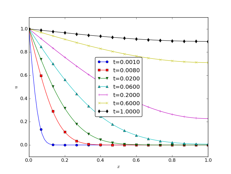
Scaled temperature in an isolated rod suddenly heated from the end

Oscillating Dirichlet condition

Now we address a heat equation problem where the temperature is oscillating on the boundary \(x=0\):

\[\tag{161} \frac{\partial u}{\partial t} = {\alpha} \frac{\partial^2 u}{\partial x^2}, \quad x\in (0,L),\ t\in (0, T],\]

\[\tag{162} u(x,0) = U_0, \quad x\in [0,L],\]

\[\tag{163} u(0, t) = U_0 + A\sin(\omega t), \quad t\in (0, T],\]

\[\tag{164} \frac{\partial}{\partial x} u(L, t) = 0, \quad t\in (0, T].\]

One important physical application is temperature oscillations in the ground, either day and night variations at a short temporal and spatial scale, or seasonal variations in the Earth’s crust. An important modeling assumption is (164), which means that the boundary \(x=L\) is placed sufficiently far from \(x=0\) such that the solution is much damped and basically constant so \(u_x=0\) is a reasonable condition.

Scaling issues

Since the boundary temperature is oscillating around the initial condition, we expect \(u\in [U_0-A,U_0+A]\). The dimensionless temperature is therefore taken as

\[\bar u = \frac{u-U_0}{A},\]

such that \(\bar u\in [-1,1]\).

What is an appropriate time scale? There will be two time scales involved, the oscillations \(\sin(\omega t)\) with period \(P=2\pi/\omega\) at the boundary and the “speed of diffusion”, or more specifically the “speed of heat conduction” in the present context, where \(t_c=x_c^2/{\alpha}\) is the appropriate scale, \(x_c\) being the length scale. Choosing the right length scale is not obvious. As we shall see, the standard choice \(x_c=L\) is not a good candidate, but to understand why, we need to examine the solution, either through simulations or through a closed-form formula. We are so lucky in this relatively simple pedagogical problem that one can find an exact solution of a related problem.

Exact solution

As usual, investigating the exact solution of the model problem can illuminate the involved scales. For this particular initial-boundary value problem the exact solution as \(t\rightarrow\infty\) (such that the initial condition \(u(x,0)=U_0\) is forgotten) and \(L\rightarrow\infty\) (such that (164) is certainly valid) can be shown to be

\[\tag{165} u(x,t) = U_0 - Ae^{-bx}\sin (bx - \omega t),\quad b =\sqrt{\frac{\omega}{2{\alpha}}}{\thinspace .}\]

This solution is of the form \(e^{-bx}g(x-ct)\), i.e., a damped wave that moves to the right with velocity \(c\) and a damped amplitude \(e^{-bx}\). This is perhaps more easily seen if we make a rewrite

\[u(x,t) = U_0 - Ae^{-bx}\sin\left(b(x - ct)\right),\quad c=\omega/b = \sqrt{2{\alpha}\omega},\ b =\sqrt{\frac{\omega}{2{\alpha}}}{\thinspace .}\]

Time and length scales

The boundary oscillations lead to the time scale \(t_c=1/\omega\). The speed of the wave suggests another time scale: the time it takes to propagate through the domain, which is \(L/c\), and hence \(t_c = L/c = L/\sqrt{2{\alpha}\omega}\).

One can argue that \(L\) is not the appropriate length scale, because \(u\) is damped by \(e^{-bx}\). So, for \(x > 4/b\), \(u\) is close to zero. We may instead use \(1/b\) as length scale, which is the e-folding distance of the damping factor, and base \(t_c\) on the time it takes a signal to propagate one length scale, \(t_c^{-1}=bc=\omega\). Similarly, the time scale based on the “speed of diffusion” changes to \(t_c^{-1}= b^2{\alpha} = \frac{1}{2}\omega\) if we employ \(1/b\) as length scale.

To summarize, we have three candidates for the time scale: \(t_c=L^2/{\alpha}\) (diffusion through the entire domain), \(t_c=2/\omega\) (diffusion through a distance \(1/b\) where \(u\) is significantly different from zero), and \(t_c=1/\omega\) (wave movement over a distance \(1/b\)).

Let us look at the dimensionless exact solution to see if it can help with the choice of scales. We introduce the dimensionless parameters

\[\beta = bx_c = x_c\sqrt{\frac{\omega}{2{\alpha}}},\quad \gamma = \omega t_c{\thinspace .}\]

The scaled solution becomes

\[\bar u(\bar x, \bar t; \beta,\gamma) = e^{-\beta\bar x}\sin(\gamma\bar t- \beta\bar x){\thinspace .}\]

The three choices of \(\gamma\), implied by the three choices of \(t_c\), are

\[\begin{split}\tag{166} \gamma = \left\lbrace\begin{array}{ll} 1, & t_c=1/\omega,\\ 2, & t_c = 2/\omega,\\ 2\beta^2, & t_c = L^2/{\alpha},\ x_c=L \end{array}\right.\end{split}\]

The former two choices leave only \(\beta\) as parameter in \(\bar u\), and with \(x_c=1/b\) as length scale, \(\beta\) becomes unity, and there are no parameters in the dimensionless solution:

\[\tag{167} \bar u(\bar x, \bar t) = e^{-\bar x}\sin(\bar t - \bar x){\thinspace .}\]

Therefore, \(x_c=1/b\) and \(t_c=1/\omega\) (or \(t_c=2/\omega\), but the factor 2 is of no importance) are the most appropriate scales.

To further argue why (167) demonstrates that these scales are preferred, think of \(\omega\) as large. Then the wave is damped over a short distance and there will be a thin boundary layer of temperature oscillations near \(x=0\) and little changes in \(u\) in the rest of the domain. The scaling (167) resolves this problem by using \(1/b \sim \omega^{-1/2}\) as length scale, because then the boundary layer thickness is independent of \(\omega\). The length of the domain can be chosen as, e.g., \(4/b\) such that \(\bar u\approx 0\) at the end \(x=L\). The length scale \(1/b\) helps us to zoom in on the part of \(u\) where significant changes take place.

In the other limit, \(\omega\) small, \(b\) becomes small, and the wave is hardly damped in the domain \([0,L]\) unless \(L\) is large enough. The imposed boundary condition on \(x=L\) in fact requires \(u\) to be approximately constant so its derivative vanishes, and this property can only be obtained if \(L\) is large enough to ensure that the wave becomes significantly damped. Therefore, the length scale is dictated by \(b\), not \(L\), and \(L\) should be adapted to \(b\), typically \(L\geq 4/b\) if \(e^{-4}\approx 0.018\) is considered enough damping to consider \(\bar u\approx 0\) for the boundary condition. This means that \(x\in [0,4/b]\) and then \(\bar x\in [0,4]\). Increasing the spatial domain to \([0,6]\) implies a damping \(e^{-6}\approx 0.0025\), if more accuracy is desired in the boundary condition.

The scaled problem

Based on the discussion of scales above, we arrive at the following scaled initial-boundary value problem:

\[\tag{168} \frac{\partial \bar u}{\partial \bar t} = \frac{1}{2}\frac{\partial^2\bar u}{\partial x^2}, \quad \bar x\in (0,4),\ \bar t\in (0,\bar T],\]

\[\tag{169} \bar u(\bar x,0) = 0, \quad \bar x\in [0,1],\]

\[\tag{170} \bar u(0,\bar t) = \sin(\bar t), \quad \bar t\in (0,\bar T],\]

\[\tag{171} \frac{\partial}{\partial\bar x}\bar u(\bar L,\bar t) = 0, \quad \bar t\in (0,\bar T].\]

The coefficient in front of the second-derivative is \(\frac{1}{2}\) because

\[\frac{t_c{\alpha}}{1/b^2} = \frac{b^2{\alpha}}{\omega} = \frac{1}{2}{\thinspace .}\]

We may, of course, choose \(t_c=2/\omega\) and get rid of the \(\frac{1}{2}\) factor, if desired, but then it turns up in (170) instead, as \(\sin (2\bar t)\).

The boundary condition at \(\bar x=\bar L\) is only an approximation and relies on sufficient damping of \(\bar u\) to consider it constant \((\partial/\partial\bar x =0)\) in space. We could, therefore, assign the condition \(\bar u = 0\) instead at \(\bar x=\bar L\).

Simulations

The file session.py contains a function solver_diffusion_FE for solving a diffusion equation in one dimension. This function can be used to solve the system (168)-(171), see diffusion_oscillatory_BC.

Diffusion wave.

Reaction-diffusion equations

Fisher’s equation

Fisher’s equation is essentially the logistic equation at each point for population dynamics (see the section Scaling a nonlinear ODE) combined with spatial movement through ordinary diffusion:

\[\tag{172} \frac{\partial u}{\partial t} = {\alpha}\frac{\partial^2 u}{\partial x^2} + \varrho u(1-u/M) {\thinspace .}\]

This PDE is also known as the KPP equation after Kolmogorov, Petrovsky, and Piskynov (who introduced the equation independently of Fisher).

Setting

\[\bar x = \frac{x}{x_c},\quad \ \bar t = \frac{t}{t_c}, \quad\bar u =\frac{u}{u_c},\]

results in

\[\frac{\partial \bar u}{\partial \bar t} = \frac{t_c{\alpha}}{x_c^2} \frac{\partial^2\bar u}{\partial\bar x^2} + t_c \varrho \bar u (1 - u_c\bar u/M){\thinspace .}\]

Balance of all terms

If all terms are equally important, the scales can be determined from demanding the coefficients to be unity. Reasoning as for the logistic ODE in the section Scaling a nonlinear ODE, we may choose \(t_c=1/\varrho\). Then the coefficient in the diffusion term dictates the length scale \(x_c = \sqrt{t_c{\alpha}}\). A natural scale for \(u\) is \(M\), since \(M\) is the upper limit of \(u\) in the model (cf. the logistic term). Summarizing,

\[u_c=M,\quad t_c = \frac{1}{\varrho},\quad x_c = \sqrt{\frac{{\alpha}}{\varrho}},\]

and the scaled PDE becomes

\[\tag{173} \frac{\partial \bar u}{\partial \bar t} = \frac{\partial^2 \bar u}{\partial\bar x^2} + \bar u (1 - \bar u){\thinspace .}\]

With this scaling, the length scale \(x_c=\sqrt{{\alpha}/\varrho}\) is not related to the domain size, so the scale is particularly relevant for infinite domains.

An open question is whether the time scale should be based on the diffusion process rather than the initial exponential growth in the logistic term. The diffusion time scale means \(t_c = x_c^2/{\alpha}\), but demanding the logistic term then to have a unit coefficient forces \(x_c^2\varrho /{\alpha} = 1\), which implies \(x_c=\sqrt{{\alpha}/\varrho}\) and \(t_c=1/\varrho\). That is, equal balance of the three terms gives a unique choice of the time and length scale.

Fixed length scale

Assume now that we fix the length scale to be \(L\), either the domain size or some other naturally given length. With \(x_c=L\), \(t_c=\varrho^{-1}\), \(u_c=M\), we get

\[\tag{174} \frac{\partial \bar u}{\partial \bar t} = \beta \frac{\partial^2 \bar u}{\partial\bar x^2} + \bar u (1 - \bar u),\]

where \(\beta\) is a dimensionless number

\[\beta = \frac{{\alpha}}{\varrho L^2} = \frac{\varrho^{-1}}{L^2/{\alpha}}{\thinspace .}\]

The last equality demonstrates that \(\beta\) measures the ratio of the time scale for exponential growth in the beginning of the logistic process and the time scale of diffusion \(L^2/{\alpha}\) (i.e., the time it takes to transport a signal by diffusion through the domain). For small \(\beta\) we can neglect the diffusion and spatial movements, and the PDE is essentially a logistic ODE at each point, while for large \(\beta\), diffusion dominates, and \(t_c\) should in that case be based on the diffusion time scale \(L^2/{\alpha}\). This leads to the scaled PDE

\[\tag{175} \frac{\partial \bar u}{\partial \bar t} = \frac{\partial^2 \bar u}{\partial\bar x^2} + \beta^{-1}\bar u (1 - \bar u),\]

showing that a large \(\beta\) encourages omission of the logistic term, because the point-wise growth takes place over long time intervals while diffusion is rapid. The effect of diffusion is then more prominent and it suffices to solve \(\bar u_{\bar t} = \bar u_{\bar x\bar x}\). The observant reader will in this latter case notice that \(u_c=M\) is an irrelevant scale for \(u\), since logistic growth with its limit is not of importance, so we implicitly assume that another scale \(u_c\) has been used, but that scale cancels anyway in the simplified PDE \(\bar u_{\bar t} = \bar u_{\bar x\bar x}\).

Nonlinear reaction-diffusion PDE

A general, nonlinear reaction-diffusion equation in 1D looks like

\[\tag{176} \frac{\partial u}{\partial t} = {\alpha}\frac{\partial^2 u}{\partial x^2} + f(u) {\thinspace .}\]

By scaling the nonlinear reaction term \(f(u)\) as \(f_c\bar f(u_c\bar u)\), where \(f_c\) is a characteristic size of \(f(u)\), typically the maximum value, one gets a non-dimensional PDE like

\[\frac{\partial\bar u}{\partial\bar t} = \frac{t_c{\alpha}}{x_c^2} \frac{\partial^2\bar u}{\partial\bar x^2} + \frac{t_cf_c}{u_c}\bar f(u_c\bar u){\thinspace .}\]

The characteristic size of \(u\) can often be derived from boundary or initial conditions, so we first assume that \(u_c\) is given. This fact uniquely determines the space and time scales by demanding that all three terms are equally important and of unit size:

\[t_c = \frac{u_c}{f_c},\quad x_c = \sqrt{\frac{{\alpha} u_c}{f_c}}{\thinspace .}\]

The corresponding PDE reads

\[\tag{177} \frac{\partial\bar u}{\partial\bar t} = \frac{\partial^2\bar u}{\partial\bar x^2} + \bar f(u_c\bar u){\thinspace .}\]

If \(x_c\) is based on some known length scale \(L\), balance of all three terms can be used to determine \(u_c\) and \(t_c\):

\[t_c = \frac{L^2}{{\alpha}},\quad u_c = \frac{L^2 f_c}{{\alpha}}{\thinspace .}\]

This scaling only works if \(f\) is nonlinear, otherwise \(u_c\) cancels and there is no freedom to constrain this scale.

With given \(L\) and \(u_c\), there are two choices of \(t_c\) since it can be based on the diffusion or the reaction time scales. With the reaction scale, \(t_c = u_c/f_c\), one arrives a the PDE

\[\tag{178} \frac{\partial\bar u}{\partial\bar t} = \beta\frac{\partial^2\bar u}{\partial\bar x^2} + \bar f(u_c\bar u),\]

where

\[\beta = \frac{{\alpha} u_c}{L^2 f_c} = \frac{u_c/f_c}{L^2/{\alpha}}\]

is a dimensionless number reflecting the ratio of the reaction time scale and the diffusion time scale. On the contrary, with the diffusion time scale, \(t_c=L^2/{\alpha}\), the scaled PDE becomes

\[\tag{179} \frac{\partial\bar u}{\partial\bar t} = \frac{\partial^2\bar u}{\partial \bar x^2} + \beta^{-1}\bar f(u_c\bar u){\thinspace .}\]

The size of \(\beta\) in an application will determine which of the scalings that is most appropriate.

The convection-diffusion equation

Convection-diffusion without a force term

We now add a convection term \(\boldsymbol{v}\cdot\nabla u\) to the diffusion equation to obtain the well-known convection-diffusion equation:

\[\tag{180} \frac{\partial u}{\partial t} + \boldsymbol{v}\cdot\nabla u = {\alpha}\nabla^2 u, \quad x,y, z\in \Omega,\ t\in (0, T]{\thinspace .}\]

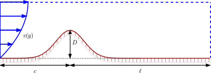
The velocity field \(\boldsymbol{v}\) is prescribed, and its characteristic size \(V\) is normally clear from the problem description. In the sketch below, we have some given flow over a bump, and \(u\) may be the concentration of some substance in the fluid. Here, \(V\) is typically \(\max_y v(y)\). The characteristic length \(L\) could be the entire domain, \(L=c+\ell\), or the height of the bump, \(L=D\). (The latter is the important length scale for the flow.)

Inserting

\[\bar x = \frac{x}{x_c},\ \bar y = \frac{y}{y_c},\ \bar z = \frac{z}{z_c}, \ \bar t = \frac{t}{t_c}, \ \bar\boldsymbol{v} = \frac{\boldsymbol{v}}{V}, \ \bar u =\frac{u}{u_c}\]

in (180) yields

\[\frac{u_c}{t_c} \frac{\partial \bar u}{\partial \bar t} + \frac{u_c V}{L}\bar\boldsymbol{v}\cdot\bar\nabla\bar u = \frac{{\alpha} u_c}{L^2}\bar\nabla^2\bar u, \quad \bar x,\bar y,\bar z\in \Omega,\ \bar t\in (0,\bar T]{\thinspace .}\]

For \(u_c\) we simply introduce the symbol \(U\), which we may estimate from an initial condition. It is not critical here, since it vanishes from the scaled equation anyway, as long as there is no source term present. With some velocity measure \(V\) and length measure \(L\), it is tempting to just let \(t_c = L/V\). This is the characteristic time it takes to transport a signal by convection through the domain. The alternative is to use the diffusion length scale \(t_c=L^2/{\alpha}\). A common physical scenario in convection-diffusion problems is that the convection term \(\boldsymbol{v}\cdot\nabla u\) dominates over the diffusion term \({\alpha}\nabla^2 u\). Therefore, the time scale for convection (\(L/V\)) is most appropriate of the two. Only when the diffusion term is very much larger than the convection term (corresponding to very small Peclet numbers, see below) \(t_c=L^2/{\alpha}\) is the right time scale.

The non-dimensional form of the PDE with \(t_c=L/V\) becomes

\[\tag{181} \frac{\partial \bar u}{\partial \bar t} + \bar\boldsymbol{v}\cdot\bar\nabla\bar u = \hbox{Pe}^{-1}\bar\nabla^2\bar u, \quad \bar x,\bar y,\bar z\in \Omega,\ \bar t\in (0,\bar T],\]

where Pe is the Peclet number,

\[\hbox{Pe} = \frac{LV}{{\alpha}}{\thinspace .}\]

Estimating the size of the convection term \(\boldsymbol{v}\cdot\nabla u\) as \(VU/L\) and the diffusion term \({\alpha}\nabla^2 u\) as \({\alpha} U/L^2\), we see that the Peclet number measures the ratio of the convection and the diffusion terms:

\[\hbox{Pe} = \frac{\hbox{convection}}{\hbox{diffusion}} = \frac{VU/L}{{\alpha} U/L^2}= \frac{LV}{{\alpha}}{\thinspace .}\]

In case we use the diffusion time scale \(t_c=L^2/{\alpha}\), we get the non-dimensional PDE

\[\tag{182} \frac{\partial \bar u}{\partial \bar t} + \hbox{Pe}\,\bar\boldsymbol{v}\cdot\bar\nabla\bar u = \bar\nabla^2\bar u, \quad \bar x,\bar y,\bar z\in \Omega,\ \bar t\in (0,\bar T]{\thinspace .}\]

Discussion of scales and balance of terms in the PDE

We see that (181) and (182) are not equal, and they are based on two different time scales. For moderate Peclet numbers around 1, all terms have the same size in (181), i.e., a size around unity. For large Peclet numbers, (181) expresses a balance between the time derivative term and the convection term, both of size unity, and then there is a very small \(\hbox{Pe}^{-1}\bar\nabla^2\bar u\) term because Pe is large and \(\bar\nabla^2\bar u\) should be of size unity. That the convection term dominates over the diffusion term is consistent with the time scale \(t_c=L/V\) based on convection transport. In this case, we can neglect the diffusion term as Pe goes to infinity and work with a pure convection (or advection) equation

\[\frac{\partial \bar u}{\partial \bar t} + \bar\boldsymbol{v}\cdot\bar\nabla\bar u = 0{\thinspace .}\]

For small Peclet numbers, \(\hbox{Pe}^{-1}\bar\nabla^2\bar u\) becomes very large and can only be balanced by two terms that are supposed to be unity of size. The time-derivative and/or the convection term must be much larger than unity, but that means we use suboptimal scales, since right scales imply that \(\partial\bar u/\partial\bar t\) and \(\bar v\cdot\bar\nabla\bar u\) are of order unity. Switching to a time scale based on diffusion as the dominating physical effect gives (182). For very small Peclet numbers this equation tells that the time-derivative balances the diffusion. The convection term \(\bar\boldsymbol{v}\cdot\bar\nabla\bar\boldsymbol{u}\) is around unity in size, but multiplied by a very small coefficient Pe, so this term is negligible in the PDE. An approximate PDE for small Peclet numbers is therefore

\[\frac{\partial \bar u}{\partial \bar t} = \bar\nabla^2\bar u{\thinspace .}\]

Scaling can, with the above type of reasoning, be used to neglect terms from a differential equation under precise mathematical conditions.

Stationary PDE

Suppose the problem is stationary and that there is no need for any time scale. How is this type of convection-diffusion problem scaled? We get

\[\frac{VU}{L}\bar\boldsymbol{v}\cdot\bar\nabla\bar u = \frac{{\alpha} U}{L^2}\bar\nabla^2\bar u,\]

or

\[\tag{183} \bar\boldsymbol{v}\cdot\bar\nabla\bar u = \hbox{Pe}^{-1}\bar\nabla^2\bar u{\thinspace .}\]

This scaling only “works” for moderate Peclet numbers. For very small or very large Pe, either the convection term \(\bar\boldsymbol{v}\cdot\bar\nabla\bar u\) or the diffusion term \(\bar\nabla^2\bar u\) must deviate significantly from unity.

Consider the following 1D example to illustrate the point: \(\boldsymbol{v} = v\boldsymbol{i}\), \(v>0\) constant, a domain \([0,L]\), with boundary conditions \(u(0)=0\) and \(u(L)=U_L\). (The vector \(\boldsymbol{i}\) is a unit vector in \(x\) direction.) The problem with dimensions is now

\[vu^{\prime} = {\alpha} u^{\prime\prime},\quad u(0)=0,\ u(L)=U_L{\thinspace .}\]

Scaling results in

\[\frac{d\bar u}{d\bar x} = \hbox{Pe}^{-1}\frac{d^2\bar u}{d\bar x^2},\quad \bar x\in (0,1),\quad \bar u(0)=0,\ \bar u(1) = 1,\]

if we choose \(U=U_L\). The solution of the scaled problem is

[ bar u(bar x) = frac{1 - e^{bar x{smallhbox{Pe}}}}{1 - e^{smallhbox{Pe}}}{thinspace .}] Figure Solution of scaled problem for 1D convection-diffusion indicates how \(\bar u\) depends on Pe: small Pe values give approximately a straight line while large Pe values lead to a boundary layer close to \(x=1\), where the solution changes very rapidly.

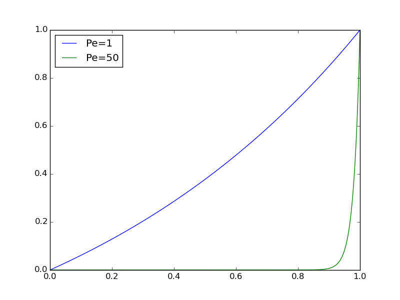
Solution of scaled problem for 1D convection-diffusion

We realize that for large Pe,

\[\max_{\bar x}\frac{d\bar u}{d\bar x} \approx \hbox{Pe},\quad \max_{\bar x}\frac{d^2\bar u}{d\bar x^2} \approx \hbox{Pe}^{2},\]

which are consistent results with the PDE, since the double derivative term is multiplied by \(\hbox{Pe}^{-1}\). For small Pe,

\[\max_{\bar x}\frac{d\bar u}{d\bar x}\approx 1,\quad \max_{\bar x}\frac{d^2\bar u}{d\bar x^2} \approx 0,\]

which is also consistent with the PDE, since an almost vanishing second-order derivative is multiplied by a very large coefficient \(\hbox{Pe}^{-1}\). However, we have a problem with very large derivatives of \(\bar u\) when Pe is large.

To arrive at a proper scaling for large Peclet numbers, we need to remove the Pe coefficient from the differential equation. There are only two scales at our disposals: \(u_c\) and \(x_c\) for \(u\) and \(x\), respectively. The natural value for \(u_c\) is the boundary value \(U_L\) at \(x=L\). The scaling of \(Vu_x = {\alpha} u_{xx}\) then results in

\[\frac{d\bar u}{d\bar x} = \frac{{\alpha}}{Vx_c}\frac{d^2\bar u}{d\bar x^2}, \quad \bar x\in (0,\bar L),\quad \bar u(0)=0,\ \bar u(\bar L)=1,\]

where \(\bar L = L/x_c\). Choosing the coefficient \({\alpha}/(Vx_c)\) to be unity results in the scale \(x_c={\alpha}/V\), and \(\bar L\) becomes Pe. The final, scaled boundary-value problem is now

\[\frac{d\bar u}{d\bar x} = \frac{d^2\bar u}{d\bar x^2}, \quad \bar x \in (0, \hbox{Pe}), \quad \bar u(0)=0,\ \bar u(\hbox{Pe})=1,\]

with solution

\[\bar u(\bar x) = \frac{1 - e^{\bar x}}{1 - e^{\small\mbox{Pe}}}{\thinspace .}\]

Figure Solution of scaled problem where the length scale depends on the Peclet number displays \(\bar u\) for some Peclet numbers, and we see that the shape of the graphs are the same with this scaling. For large Peclet numbers we realize that \(\bar u\) and its derivatives are around unity (\(1-e^{\hbox{Pe}}\approx -e^{\small\hbox{Pe}}\)), but for small Peclet numbers \(d\bar u/d\bar x \sim \hbox{Pe}^{-1}\).

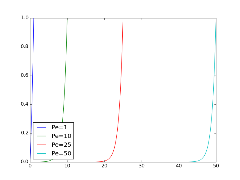
Solution of scaled problem where the length scale depends on the Peclet number

The conclusion is that for small Peclet numbers, \(x_c=L\) is an appropriate length scale. The scaled equation \(\hbox{Pe}\,\bar u' = \bar u''\) indicates that \(\bar u''\approx 0\), and the solution is close to a straight line. For large Pe values, \(x_c={\alpha}/V\) is an appropriate length scale, and the scaled equation \(\bar u' = \bar u''\) expresses that the terms \(\bar u'\) and \(\bar u''\) are equal and of size around unity.

Convection-diffusion with a source term

Let us add a force term \(f(\boldsymbol{x},t)\) to the convection-diffusion equation:

\[\tag{184} \frac{\partial u}{\partial t} + \boldsymbol{v}\cdot\nabla u = {\alpha}\nabla^2 u + f{\thinspace .}\]

The scaled version reads

\[\frac{\partial\bar u}{\partial\bar t} + \frac{t_cV}{L}\bar\boldsymbol{v}\cdot\bar\nabla \bar u = \frac{t_c{\alpha}}{L^2}\bar\nabla^2 \bar u + \frac{t_cf_c}{u_c}\bar f{\thinspace .}\]

We can base \(t_c\) on convective transport: \(t_c = L/V\). Now, \(u_c\) could be chosen to make the coefficient in the source term unity: \(u_c = t_cf_c = Lf_c/V\). This leaves us with

\[\frac{\partial\bar u}{\partial\bar t} + \bar\boldsymbol{v}\cdot\bar \nabla\bar u = \hbox{Pe}^{-1}\bar \nabla^2 \bar u + \bar f{\thinspace .}\]

In the diffusion limit, we base \(t_c\) on the diffusion time scale: \(t_c=L^2/{\alpha}\), and the coefficient of the source term set to unity determines \(u_c\) according to

\[\frac{L^2 f_c}{{\alpha} u_c} = 1\quad\Rightarrow\quad u_c = \frac{L^2 f_c}{{\alpha}}{\thinspace .}\]

The corresponding PDE reads

\[\frac{\partial\bar u}{\partial\bar t} + \hbox{Pe}\,\bar\boldsymbol{v}\cdot\bar \nabla\bar u = \bar\nabla^2 \bar u + \bar f,\]

so for small Peclet numbers, which we have, the convective term can be neglected and we get a pure diffusion equation with a source term.

What if the problem is stationary? Then there is no time scale and we get

\[\frac{V u_c}{L}\bar\boldsymbol{v}\cdot\bar \nabla \bar u = \frac{u_c {\alpha}}{L^2}\bar\nabla^2 \bar u + f_c\bar f,\]

or

\[\bar\boldsymbol{v}\cdot\bar \nabla \bar u = \hbox{Pe}^{-1}\bar\nabla^2 \bar u + \frac{f_c L}{V u_c}\bar f{\thinspace .}\]

Again, choosing \(u_c\) such that the source term coefficient is unity leads to \(u_c= f_c L/V\). Alternatively, \(u_c\) can be based on the initial condition, with similar results as found in the sections on the wave and diffusion PDEs.

Exercises

Problem 3.1: Stationary Couette flow

A fluid flows between two flat plates, with one plate at rest while the other moves with velocity \(U_0\). This classical flow case is known as stationary Couette flow.

a) Directing the \(x\) axis in the flow direction and letting \(y\) be a coordinate perpendicular to the walls, one can assume that the velocity field simplifies to \(\boldsymbol{u} = u(y)\boldsymbol{i}\). Show from the Navier-Stokes equations that the boundary-value problem for \(u(y)\) is

\[u^{\prime\prime}(u) = 0,\quad u(0)=0,\ u(H)=U_0{\thinspace .}\]

We have here assumed at \(y=0\) corresponds to the plate at rest and that \(y=H\) represents the plate that moves. There are no pressure gradients present in the flow.

b) Scale the problem in a) and show that the result has no physical parameters left in the model:

\[\frac{d^2\bar u}{d\bar y^2} = 0,\quad \bar u(0)=0,\ \bar u(1)=1{\thinspace .}\]

c) We can compute \(\bar u(\bar y)\) from one numerical simulation (or a straightforward integration of the differential equation). Set up the formula that finds \(u(y; H, u_0)\) from \(\bar u(\bar y)\) for any values of \(H\) and \(U_0\).

Filename: stationary_Couette.

Remarks

The problem for \(u\) is a classical two-point boundary-value problem in applied mathematics and arises in a number of applications, where Couette flow is just one example. Heat conduction is another example: \(u\) is temperature, and the heat conduction equation for an insulated rod reduces to \(u^{\prime\prime}=0\) under stationary conditions and no heat source. Controlling the end \(x=0\) at 0 degrees Celsius the other end \(x=L\) at \(U_0\) degrees Celsius, gives the same boundary conditions as in the above flow problem. The scaled problem is of course the same whether we have flow of fluid or heat.

Exercise 3.2: Couette-Poiseuille flow

Viscous fluid flow between two infinite flat plates \(z=0\) and \(z=H\) is governed by

\[\tag{185} \mu u''(z) = -\beta\]

\[\tag{186} u(0) = 0,\]

\[\tag{187} u(H) = U_0{\thinspace .}\]

Here, \(u(z)\) is the fluid velocity in \(x\) direction (perpendicular to the \(z\) axis), \(\mu\) is the dynamic viscosity of the fluid, \(\beta\) is a positive constant pressure gradient, and \(U_0\) is the constant velocity of the upper plate \(z=H\) in \(x\) direction. The model represents Couette flow for \(\beta=0\) and Poiseuille flow for \(U_0=0\).

a) Find the exact solution \(u(z)\). Point out how \(\beta\) and \(U_0\) influence the magnitude of \(u\).

b) Scale the problem.

Filename: Couette_wpressure.

Exercise 3.3: Pulsatile pipeflow

The flow of a viscous fluid in a straight pipe with circular cross section with radius \(R\) is governed by

\[\tag{188} \varrho\frac{\partial u}{\partial t} = \frac{\mu}{r}\frac{\partial}{\partial r} \left(r\frac{\partial u}{\partial r}\right) - P(t), r\in (0,R),\ t\in (0,T],\]

\[\tag{189} \frac{\partial u}{\partial r}(0,t) = 0, t\in (0,T],\]

\[\tag{190} u(R,t) = 0, t\in (0,T],\]

\[\tag{191} u(r,0) = 0, r\in [0,R].\]

The quantity \(u(r,t)\) is the fluid velocity, \(P(t)\) is a given pressure gradient, \(\varrho\) is the fluid density, and \(\mu\) is the dynamic viscosity.

Assume \(P(t) = A\cos\omega t\). Scale the problem and identify appropriate dimensionless numbers. Thereafter, assume \(P(t)\) is a more complicated function, but still period with period \(p\). Discuss how the scaling can be extended to this case.

Filename: pipeflow.

Exercise 3.4: The linear cable equation

A key PDE in neuroscience is the cable equation, here given in its simplest linear form:

\[\tag{192} \tau\frac{\partial u}{\partial t} = \lambda^2\frac{\partial^2 u}{\partial x^2} -u{\thinspace .}\]

The unknown \(u\) is the voltage (measured in volt) associated with an electric current along one-dimensional dendrites (“cables”) in neural networks, while \(\tau\) and \(\lambda\) are given parameters.

Scale (192) in three ways: 1) let all terms in the scaled equation have unit coefficients, 2) use the domain size \(L\) as spatial scale and base the time scale on diffusion, 3) use the domain size \(L\) as spatial scale and base the time scale on reaction, i.e., the \(-u\) term.

Filename: cable_eq.

Exercise 3.5: Heat conduction with discontinuous initial condition

Two pieces of metal at different temperature are brought in contact at \(t=0\). The following initial-boundary value problem governs the temperature evolution in the two pieces:

\[\tag{193} \frac{\partial u}{\partial t} = {\alpha}\nabla^2 u,\ \boldsymbol{x}\in\Omega,\ t\in (0,T],\]

\[\tag{194} u(\boldsymbol{x},0)=I(x), \boldsymbol{x}\in \Omega,\]

\[\tag{195} -{\alpha}\frac{\partial u}{\partial n} = h(u-u_S), x\in\partial\Omega,\ t\in (0,T].\]

Here, \(u(\boldsymbol{x},t)\) is the temperature, \({\alpha}\) the effective heat diffusion coefficient (assuming both pieces are homogeneous and of the same type of metal), and \(u_S\) is the surrounding temperature. The domain \(\Omega\) consists of the two pieces \(\Omega_1\) and \(\Omega_2\): \(\Omega = \Omega_1\cup\Omega_2\). The initial condition can be specified as

\[\begin{split}I(x) = \left\lbrace\begin{array}{ll} U_1, & \boldsymbol{x}\in\Omega_1,\\ U_2, & \boldsymbol{x}\in\Omega_2, \end{array}\right.\end{split}\]

where \(U_1\) and \(U_2\) are the constant initial temperatures in each piece.

Thinking of two identical pieces \(\Omega_1\) and \(\Omega_2\) with shapes as bricks, it is tempting to develop a one-dimensional model, especially if the pieces are somewhat slender. We then expect the main temperature variations to take place in the \(x\) direction, where the \(x\) axis is perpendicular to the contact surface between the pieces. A simplified PDE problem, neglecting variations in the \(y\) and \(z\) directions, takes the form

\[\tag{196} \frac{\partial v}{\partial t} = {\alpha} \frac{\partial^2 v}{\partial x^2} -\frac{hP}{A}(v(x,t) -u_S),\ x\in (0,L),\ t\in (0,T],\]

\[\tag{197} v(x,0)=I(x), x\in (0,L),\]

\[\tag{198} {\alpha}\frac{\partial v}{\partial x} = h(v(x,t)-u_S), x=0,\ t\in (0,T],\]

\[\tag{199} -{\alpha}\frac{\partial v}{\partial x} = h(v(x,t)-u_S), x=L,\ t\in (0,T],\]

with

\[\begin{split}I(x) = \left\lbrace\begin{array}{ll} U_1, & x\in [0,L/2),\\ U_2, & x\in [L/2, L]{\thinspace .} \end{array}\right.\end{split}\]

The parameter \(P\) is the perimeter of the cross section and \(A\) is the area of the cross section. Scale this problem.

Filename: metal_pieces.

Remarks

We can derive (196)-(199) from (194)-(195). The idea is to integrate the governing PDE (196) in the two directions where we expect negligible variations, use the Gauss divergence theorem in these directions, and apply the cooling boundary condition. Let \(A\) be the cross section of the bricks. Integrating over \(A\) gives

\[\begin{split}\int\limits_A \frac{\partial u}{\partial t}dydz &= \int\limits_A {\alpha}\left( \frac{\partial^2 u}{\partial x^2} + \frac{\partial^2 u}{\partial y^2} + \frac{\partial^2 u}{\partial z^2} \right)dydz \\ &=\int\limits_A {\alpha} \frac{\partial^2 u}{\partial x^2} dydz + \int\limits_A {\alpha}\left( \frac{\partial^2 u}{\partial y^2} + \frac{\partial^2 u}{\partial z^2} \right)dydz \\ & = \int\limits_A {\alpha} \frac{\partial^2 u}{\partial x^2} dydz + {\alpha}\int\limits_{\partial A}\frac{\partial u}{\partial n}ds\\ & = \int\limits_A {\alpha} \frac{\partial^2 u}{\partial x^2} dydz -h(v(x,t) -u_S)P{\thinspace .}\end{split}\]

The parameter \(P\) is the perimeter of the cross section \(A\). The function \(v(x,t)\) means \(u(\boldsymbol{x},t)\) evaluated at the boundary \(\partial A\). Assuming \(u\) to vary little across the cross section \(A\), we can approximate the integrals by \(u\) evaluated at \(\partial A\) as \(v\):

\[\int\limits_A \frac{\partial u}{\partial t}dydz\approx A \frac{\partial}{\partial t} v(x,t), \quad \int\limits_A {\alpha} \frac{\partial^2 u}{\partial x^2} dydz \approx A {\alpha} \frac{\partial^2 v}{\partial x^2},\]

where \(A\) now is the cross-section area. The result is the 1D initial-boundary value problem (196)-(199).

Problem 3.6: Scaling a welding problem

Welding equipment makes a very localized heat source that moves in time. We shall investigate the heating due to welding and choose, for maximum simplicity, a one-dimensional heat equation with a fixed temperature at the ends (a 2D or 3D model with cooling conditions at the boundaries would be of greater physical significance, but now the scaling is in focus). The effect of melting is not included in the heat equation. Our goal is to investigate two alternative scalings through numerical experimentation.

The governing PDE problem reads

\[\begin{split}\varrho c\frac{\partial u}{\partial t} &= k\frac{\partial^2 u}{\partial x^2} + f, & x\in (0,L),\ t\in (0,T),\\ u(x,0) &= U_s, & x\in [0,L],\\ u(0,t) = u(L,t) &= U_s, & t\in (0,T].\end{split}\]

Here, \(u\) is the temperature, \(\varrho\) the density of the material, \(c\) a heat capacity, \(k\) the heat conduction coefficient, \(f\) is the heat source from the welding equipment, and \(U_s\) is the initial constant (room) temperature in the material.

A possible model for the heat source is a moving Gaussian function:

\[f = A\exp{\left(-\frac{1}{2}\left(\frac{x-vt}{\sigma}\right)^2\right)},\]

where \(A\) is the strength, \(\sigma\) is a parameter governing how peak-shaped (or localized in space) the heat source is, and \(v\) is the velocity (in positive \(x\) direction) of the source.

a) Let \(x_c\), \(t_c\), \(u_c\), and \(f_c\) be scales, i.e., characteristic sizes, of \(x\), \(t\), \(u\), and \(f\), respectively. The natural choice of \(x_c\) and \(f_c\) is \(L\) and \(A\), since these make the scaled \(x\) and \(f\) in the interval \([0,1]\). If each of the three terms in the PDE are equally important, we can find \(t_c\) and \(u_c\) by demanding that the coefficients in the scaled PDE are all equal to unity. Perform this scaling. Use scaled quantities in the arguments for the exponential function in \(f\) too and show that

\[\bar f= \exp{\left(-\frac{1}{2}\beta^2(\bar x -\gamma \bar t)^2\right)},\]

where \(\beta\) and \(\gamma\) are dimensionless numbers. Give an interpretation of \(\beta\) and \(\gamma\).

b) Argue that at least for large \(\gamma\) we should base the time scale on the movement of the heat source. Using \(L\) as length scale, show that this gives rise to the scaled PDE

\[\frac{\partial\bar u}{\partial\bar t} = \gamma^{-1}\frac{\partial^2\bar u}{\partial\bar x^2} + \bar f,\]

and

\[\bar f = \exp{(-\frac{1}{2}\beta^2(\bar x - \bar t)^2)}{\thinspace .}\]

Discuss when the scalings in a) and b) are appropriate.

c) For fast movement of the welding equipment, i.e., when heat transfer is less important than the local heating by the equipment, the typical length scale of the local heating is the size of the source, reflected by the \(\sigma\) parameter. Modify the scaling in b) when \(\sigma\) is chosen as length scale.

d) A fourth kind of possible scaling is to say that for small \(\gamma\), the problem is quasi-stationary and the heat transfer balances the heat source. Determine \(u_c\) from this assumption. Use \(L\) as length scale and a time scale as in b), i.e., based on the movement of the welding equipment.

e) One aim with scaling is to get a solution that lies in the interval \([-1,1]\). This is not always the case when \(u_c\) is based on a scale involving a source term, as we do in a)-c). However, from the scaled PDE we realize that if we replace \(\bar f\) with \(\delta\bar f\), where \(\delta\) is a dimensionless factor, this corresponds to replacing \(u_c\) by \(u_c/\delta\). So, if we observe that \(\bar u\sim1/\delta\) in simulations, we can just replace \(\bar f\) by \(\delta \bar f\) in the scaled PDE.

Use this trick and implement the four scaled models in a)-d). Reuse some software for the 1D diffusion equation. Make a function run(gamma, beta=10, delta=40, scaling=1, animate=False) that runs an implementation of the unscaled model with the given \(\gamma\), \(\beta\), and \(\delta\) parameters as well as an indicator scaling that is 'a', 'b', and so forth. The last argument can be used to turn screen animations on or off.

Perform experiments to find the proper value of \(\delta\) for each \(\gamma\) and for each scaling.

Equip the run function with visualization, both animation of \(\bar u\) and \(\bar f\), and plots with \(\bar u\) and \(\bar f\) for \(t=0.2\) and \(t=0.5\).

Hint. Since the amplitudes of \(\bar u\) and \(\bar f\) differs by a factor \(\delta\), it is attractive to plot \(\bar f/\delta\) together with \(\bar u\).

f) Use the software in e) to investigate \(\gamma=0.2,1,5,40\) for the four scalings. Discuss the results.

Filename: welding.