
The goal of this chapter is to show how the Poisson equation, the most basic of all PDEs, can be quickly solved with a few lines of FEniCS code. We introduce the most fundamental FEniCS objects such asMesh,Function,FunctionSpace,TrialFunction, andTestFunction, and learn how to write a basic PDE solver, including the specification of the mathematical variational problem, applying boundary conditions, calling the FEniCS solver, and plotting the solution.
Most books on a programming language start with a “Hello, World!” program. That is, one is curious about how a very fundamental task is expressed in the language, and writing a text to the screen can be such a task. In the world of finite element methods for PDEs, the most fundamental task must be to solve the Poisson equation. Our counterpart to the classical “Hello, World!” program therefore solves
Here, \(u = u(\boldsymbol{x})\) is the unknown function, \(f = f(\boldsymbol{x})\) is a prescribed function, \(\nabla^2\) is the Laplace operator (also often written as \(\Delta\)), \(\Omega\) is the spatial domain, and \(\partial\Omega\) is the boundary of \(\Omega\). A stationary PDE like this, together with a complete set of boundary conditions, constitute a boundary-value problem, which must be precisely stated before it makes sense to start solving it with FEniCS.
In two space dimensions with coordinates \(x\) and \(y\), we can write out the Poisson equation as
The unknown \(u\) is now a function of two variables, \(u = u(x,y)\), defined over a two-dimensional domain \(\Omega\).
The Poisson equation arises in numerous physical contexts, including heat conduction, electrostatics, diffusion of substances, twisting of elastic rods, inviscid fluid flow, and water waves. Moreover, the equation appears in numerical splitting strategies for more complicated systems of PDEs, in particular the Navier - Stokes equations.
Solving a PDE such as the Poisson equation in FEniCS consists of the following steps:
- Identify the computational domain (\(\Omega\)), the PDE, its boundary conditions, and source terms (\(f\)).
- Reformulate the PDE as a finite element variational problem.
- Write a Python program which defines the computational domain, the variational problem, the boundary conditions, and source terms, using the corresponding FEniCS abstractions.
- Call FEniCS to solve the PDE and, optionally, extend the program to compute derived quantities such as fluxes and averages, and visualize the results.
We shall now go through steps 2 - 4 in detail. The key feature of FEniCS is that steps 3 and 4 result in fairly short code, while a similar program in most other software frameworks for PDEs require much more code and more technically difficult programming.
What makes FEniCS attractive
Although many frameworks have a really elegant “Hello, World!” example on the Poisson equation, FEniCS is to our knowledge the only framework where the code stays compact and nice, very close to the mathematical formulation, also when the complexity increases with, e.g., systems of PDEs and mixed finite elements for computing on massively high-performance parallel platforms.
FEniCS is based on the finite element method, which is a general and efficient mathematical machinery for numerical solution of PDEs. The starting point for the finite element methods is a PDE expressed in variational form. Readers who are not familiar with variational problems will get a very brief introduction to the topic in this tutorial, but reading a proper book on the finite element method in addition is encouraged. The section The finite element method contains a list of some suitable books. Experience shows that you can work with FEniCS as a tool to solve your PDEs even without thorough knowledge of the finite element method, as long as you get somebody to help you with formulating the PDE as a variational problem.
The basic recipe for turning a PDE into a variational problem is to multiply the PDE by a function \(v\), integrate the resulting equation over the domain \(\Omega\), and perform integration by parts of terms with second-order derivatives. The function \(v\) which multiplies the PDE is called a test function. The unknown function \(u\) to be approximated is referred to as a trial function. The terms test and trial function are used in FEniCS programs too. Suitable function spaces must be specified for the test and trial functions. For standard PDEs arising in physics and mechanics such spaces are well known.
In the present case, we first multiply the Poisson equation by the test function \(v\) and integrate over \(\Omega\):
A common rule when we derive variational formulations is that we try to keep the order of the derivatives of \(u\) and \(v\) as low as possible (this will enlarge the collection of finite elements that can be used in the problem). Here, we have a second-order spatial derivative of \(u\), which can be transformed to a first-derivative of \(u\) and \(v\) by applying the technique of integration by parts. A Laplace term will always be subject to integration by parts [1]. The formula reads
where \(\frac{\partial u}{\partial n} = \nabla u \cdot n\) is the derivative of \(u\) in the outward normal direction \(n\) on the boundary.
| [1] | Integration by parts in more than one space dimension is based on Gauss’ divergence theorem. Simply take (5) as the formula to be used. |
Another feature of variational formulations is that the test function \(v\) is required to vanish on the parts of the boundary where the solution \(u\) is known (the book [Ref10] explains in detail why this requirement is necessary). In the present problem, this means that \(v=0\) on the whole boundary \(\partial\Omega\). The second term on the right-hand side of (5) therefore vanishes. From (4) and (5) it follows that
If we require that this equation holds for all test functions \(v\) in some suitable space \(\hat V\), the so-called test space, we obtain a well-defined mathematical problem that uniquely determines the solution \(u\) which lies in some (possibly different) function space \(V\), the so-called trial space. We refer to (6) as the weak form or variational form of the original boundary-value problem (1)–(2).
The proper statement of our variational problem now goes as follows: Find \(u \in V\) such that
The trial and test spaces \(V\) and \(\hat V\) are in the present problem defined as
In short, \(H^1(\Omega)\) is the mathematically well-known Sobolev space containing functions \(v\) such that \(v^2\) and \(|\nabla v|^2\) have finite integrals over \(\Omega\) (essentially meaning that the functions are continuous). The solution of the underlying PDE must lie in a function space where also the derivatives are continuous, but the Sobolev space \(H^1(\Omega)\) allows functions with discontinuous derivatives. This weaker continuity requirement of \(u\) in the variational statement (7), as a result of the integration by parts, has great practical consequences when it comes to constructing finite element function spaces. In particular, it allows the use of piecewise polynomial function spaces; i.e., function spaces constructed by stitching together polynomial functions on simple domains such as intervals, triangles, or tetrahedrons.
The variational problem (7) is a continuous problem: it defines the solution \(u\) in the infinite-dimensional function space \(V\). The finite element method for the Poisson equation finds an approximate solution of the variational problem (7) by replacing the infinite-dimensional function spaces \(V\) and \(\hat{V}\) by discrete (finite-dimensional) trial and test spaces \(V_h\subset{V}\) and \(\hat{V}_h\subset\hat{V}\). The discrete variational problem reads: Find \(u_h \in V_h \subset V\) such that
This variational problem, together with a suitable definition of the function spaces \(V_h\) and \(\hat{V}_h\), uniquely define our approximate numerical solution of Poisson’s equation (1). The mathematical framework may seem complicated at first glance, but the good news is that the finite element variational problem (8) looks the same as the continuous variational problem (7), and FEniCS can automatically solve variational problems like (8)!
What we mean by the notation \(u\) and \(V\)
The mathematics literature on variational problems writes \(u_h\) for the solution of the discrete problem and \(u\) for the solution of the continuous problem. To obtain (almost) a one-to-one relationship between the mathematical formulation of a problem and the corresponding FEniCS program, we shall drop the subscript \(_h\) and use \(u\) for the solution of the discrete problem and \({u_{\small\mbox{e}}}\) for the exact solution of the continuous problem, if we need to explicitly distinguish between the two. Similarly, we will let \(V\) denote the discrete finite element function space in which we seek our solution.
It turns out to be convenient to introduce the following canonical notation for variational problems:
For the Poisson equation, we have:
From the mathematics literature, \(a(u,v)\) is known as a bilinear form and \(L(v)\) as a linear form. We shall in every linear problem we solve identify the terms with the unknown \(u\) and collect them in \(a(u,v)\), and similarly collect all terms with only known functions in \(L(v)\). The formulas for \(a\) and \(L\) are then coded directly in the program.
FEniCS provides all the necessary mathematical notation needed to express the variational problem \(a(u, v) = L(v)\). To solve a linear PDE in FEniCS, such as the Poisson equation, a user thus needs to perform only two steps:
- Choose the finite element spaces \(V\) and \(\hat V\) by specifying the domain (the mesh) and the type of function space (polynomial degree and type).
- Express the PDE as a (discrete) variational problem: find \(u\in V\) such that \(a(u,v) = L(v)\) for all \(v\in \hat{V}\).
The Poisson problem (1)–(2) has so far featured a general domain \(\Omega\) and general functions \(u_{_\mathrm{D}}\) for the boundary conditions and \(f\) for the right-hand side. For our first implementation we will need to make specific choices for \(\Omega\), \(u_{_\mathrm{D}}\), and \(f\). It will be wise to construct a problem where we can easily check that the computed solution is correct. Solutions that are lower-order polynomials are primary candidates. Standard finite element function spaces of degree \(r\) will exactly reproduce polynomials of degree \(r\). And piecewise linear elements (\(r=1\)) are able to exactly reproduce a quadratic polynomial on a uniformly partitioned mesh. This important result can be used to verify our implementation. We just manufacture some quadratic function in 2D as the exact solution, say
By inserting (12) into the Poisson equation (1), we find that \({u_{\small\mbox{e}}}(x,y)\) is a solution if
regardless of the shape of the domain as long as \({u_{\small\mbox{e}}}\) is prescribed along the boundary. We choose here, for simplicity, the domain to be the unit square,
This simple but very powerful method for constructing test problems is called the method of manufactured solutions: pick a simple expression for the exact solution, plug it into the equation to obtain the right-hand side (source term \(f\)), then solve the equation with this right-hand side and try to reproduce the exact solution.
Tip: Try to verify your code with exact numerical solutions
A common approach to testing the implementation of a numerical method is to compare the numerical solution with an exact analytical solution of the test problem and conclude that the program works if the error is “small enough”. Unfortunately, it is impossible to tell if an error of size \(10^{-5}\) on a \(20\times 20\) mesh of linear elements is the expected (in)accuracy of the numerical approximation or if the error also contains the effect of a bug in the code. All we usually know about the numerical error is its asymptotic properties, for instance that it is proportional to \(h^2\) if \(h\) is the size of a cell in the mesh. Then we can compare the error on meshes with different \(h\)-values to see if the asymptotic behavior is correct. This is a very powerful verification technique and is explained in detail in the section Computing convergence rates. However, if we have a test problem for which we know that there should be no approximation errors, we know that the analytical solution of the PDE problem should be reproduced to machine precision by the program. That is why we emphasize this kind of test problems throughout this tutorial. Typically, elements of degree \(r\) can reproduce polynomials of degree \(r\) exactly, so this is the starting point for constructing a solution without numerical approximation errors.
A FEniCS program for solving our test problem for the Poisson equation in 2D with the given choices of \(u_{_\mathrm{D}}\), \(f\), and \(\Omega\) may look as follows:
from fenics import *

# Create mesh and define function space
mesh = UnitSquareMesh(8, 8)
V = FunctionSpace(mesh, 'P', 1)

# Define boundary condition
u_D = Expression('1 + x[0]*x[0] + 2*x[1]*x[1]', degree=2)

def boundary(x, on_boundary):
    return on_boundary

bc = DirichletBC(V, u_D, boundary)

# Define variational problem
u = TrialFunction(V)
v = TestFunction(V)
f = Constant(-6.0)
a = dot(grad(u), grad(v))*dx
L = f*v*dx

# Compute solution
u = Function(V)
solve(a == L, u, bc)

# Plot solution
u.rename('u', 'solution')
plot(u)
plot(mesh)

# Save solution to file in VTK format
vtkfile = File('poisson.pvd')
vtkfile << u

# Compute error in L2 norm
error_L2 = errornorm(u_D, u, 'L2')

# Compute maximum error at vertices
vertex_values_u_D = u_D.compute_vertex_values(mesh)
vertex_values_u = u.compute_vertex_values(mesh)
import numpy as np
error_max = np.max(np.abs(vertex_values_u_D - vertex_values_u))

# Print errors
print('error_L2  =', error_L2)
print('error_max =', error_max)

# Hold plot
interactive()
The complete code can be found in the file ft01_poisson.py.
The FEniCS program must be available in a plain text file, written with a text editor such as Atom, Sublime Text, Emacs, Vim, or similar.
There are several ways to run a Python program like
ft01_poisson.py:
- Use a terminal window.
- Use an integrated development environment (IDE), e.g., Spyder.
- Use a Jupyter notebook.
Open a terminal window, move to the directory containing the program and type the following command:
Terminal> python ft01_poisson.py
Note that this command must be run in a FEniCS-enabled terminal. For
users of the FEniCS Docker containers, this means that you must type
this command after you have started a FEniCS session using
fenicsproject run or fenicsproject start.
When running the above command, FEniCS will run the program to compute the approximate solution \(u\). The approximate solution \(u\) will be compared to the exact solution \({u_{\small\mbox{e}}}\) and the error in the \(L^2\) and maximum norms will be printed. Since we know that our approximate solution should reproduce the exact solution to within machine precision, this error should be small, something on the order of \(10^{-15}\).
Plot of the solution in the first FEniCS example
Many prefer to work in an integrated development environment that
provides an editor for programming, a window for executing code, a
window for inspecting objects, etc. The Spyder tool comes with all
major Python installations. Just open the file ft01_poisson.py
and press the play button to run it. We refer to the Spyder tutorial
to learn more about working in the Spyder environment. Spyder is
highly recommended if you are used to working in the graphical
MATLAB environment.
Notebooks make it possible to mix text and executable code in the same
document, but you can also just use it to run programs in a web browser.
Start jupyter notebook from a terminal window, find the New pulldown
menu in the upper right part of the GUI, choose a new notebook in
Python 2 or 3, write %load ft01_poisson.py in the blank
cell of this notebook, then press Shift+Enter to execute the cell.
The file ft01_poisson.py will then be loaded into the notebook.
Re-execute the cell (Shift+Enter) to run the program. You may divide the
entire program into several cells to examine intermediate results: place
the cursor where you want to split the cell and choose Edit - Split Cell.
We shall now dissect our FEniCS program in detail. The listed FEniCS program defines a finite element mesh, a finite element function space \(V\) on this mesh, boundary conditions for \(u\) (the function \(u_{_\mathrm{D}}\)), and the bilinear and linear forms \(a(u,v)\) and \(L(v)\). Thereafter, the unknown trial function \(u\) is computed. Then we can compare the numerical and exact solution as well as visualize the computed solution \(u\).
The first line in the program,
from fenics import *
imports the key classes UnitSquareMesh, FunctionSpace, Function,
and so forth, from the FEniCS library. All FEniCS programs for
solving PDEs by the finite element method normally start with this
line.
The statement
mesh = UnitSquareMesh(8, 8)
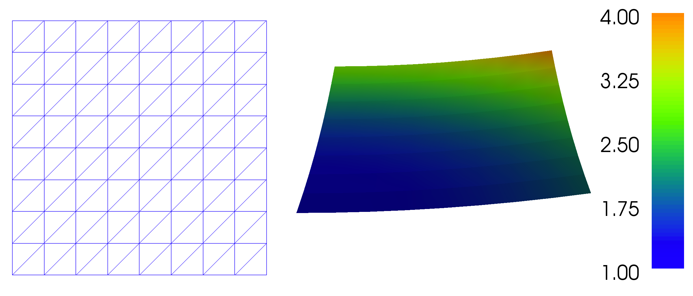
defines a uniform finite element mesh over the unit square \([0,1]\times [0,1]\). The mesh consists of cells, which in 2D are triangles with straight sides. The parameters 8 and 8 specify that the square should be divided into \(8\times 8\) rectangles, each divided into a pair of triangles. The total number of triangles (cells) thus becomes 128. The total number of vertices in the mesh is \(9\cdot 9=81\). In later chapters, you will learn how to generate more complex meshes.
Having a mesh, we can define a finite element function space V over
this mesh:
V = FunctionSpace(mesh, 'P', 1)
The second argument 'P‘ specifies the type of element, while the third
argument is the degree of the basis functions of the element. The type
of element is here \(\mathsf{P}\), implying the standard Lagrange family of
elements. You may also use 'Lagrange' to specify this type of
element. FEniCS supports all simplex element families and the notation
defined in the Periodic Table of the Finite Elements [Ref22].
The third argument 1 specifies the degree of the finite element. In
this case, the standard \(\mathsf{P}_1\) linear Lagrange element, which
is a triangle with nodes at the three vertices. Some finite element
practitioners refer to this element as the “linear triangle”. The
computed solution \(u\) will be continuous and linearly varying in \(x\)
and \(y\) over each cell in the mesh. Higher-degree polynomial
approximations over each cell are trivially obtained by increasing the
third parameter to FunctionSpace, which will then generate function
spaces of type \(\mathsf{P}_2\), \(\mathsf{P}_3\), and so forth.
Changing the second parameter to 'DP' creates a function
space for discontinuous Galerkin methods.
In mathematics, we distinguish between the trial and test spaces \(V\)
and \(\hat{V}\). The only difference in the present problem is the
boundary conditions. In FEniCS we do not specify the boundary
conditions as part of the function space, so it is sufficient to work
with one common space V for the trial and test functions in the
program:
u = TrialFunction(V)
v = TestFunction(V)
The next step is to specify the boundary condition: \(u=u_{_\mathrm{D}}\) on \(\partial\Omega\). This is done by
bc = DirichletBC(V, u_D, boundary)
where u_D is an expression defining the solution values on the
boundary, and boundary is a function (or object) defining
which points belong to the boundary.
Boundary conditions of the type \(u=u_{_\mathrm{D}}\) are known as Dirichlet
conditions. For the present finite element method for the Poisson
problem, they are also called essential boundary conditions, as they
need to be imposed explicitly as part of the trial space (in contrast
to being defined implicitly as part of the variational formulation).
Naturally, the FEniCS class used to define Dirichlet boundary
conditions is named DirichletBC.
The variable u_D refers to an Expression object, which is used to
represent a mathematical function. The typical construction is
u_D = Expression(formula, degree=1)
where formula is a string containing the mathematical expression.
This formula is written with C++ syntax. The expression is
automatically turned into an efficient, compiled C++ function.
The second argument degree is a parameter that specifies how
the expression should be treated in computations. FEniCS will
interpolate the expression into some finite element space. It is
usually a good choice to interpolate expressions into the same
space \(V\) that is used for the trial and test functions,
but in certain cases, one may want to use a more accurate (higher
degree) representation of expressions.
The expression may depend on the variables x[0] and x[1]
corresponding to the \(x\) and \(y\) coordinates. In 3D, the expression
may also depend on the variable x[2] corresponding to the \(z\)
coordinate. With our choice of \(u_{_\mathrm{D}}(x,y)=1 + x^2 + 2y^2\), the formula
string can be written as 1 + x[0]*x[0] + 2*x[1]*x[1]:
u_D = Expression('1 + x[0]*x[0] + 2*x[1]*x[1]', degree=2)
We set the degree to \(2\) so that u_D may represent the exact
quadratic solution to our test problem.
[hpl 1: What do you do with a really smooth function line \(sin(x)\)? What degree? Why not a default degree? This is difficult for a beginner.]
String expressions must have valid C++ syntax
The string argument to an Expression object must obey C++ syntax.
Most Python syntax for mathematical expressions is also valid C++ syntax,
but power expressions make an exception: p**a must be written as
pow(p, a) in C++ (this is also an alternative Python syntax).
The following mathematical functions can be used directly
in C++
expressions when defining Expression objects:
cos, sin, tan, acos, asin,
atan, atan2, cosh, sinh, tanh, exp,
frexp, ldexp, log, log10, modf,
pow, sqrt, ceil, fabs, floor, and fmod.
Moreover, the number \(\pi\) is available as the symbol pi.
All the listed functions are taken from the cmath C++ header file, and
one may hence
consult the documentation of cmath for more information on the
various functions.
If/else tests are possible using the C syntax for inline branching. The function
is implemented as
f = Expression('x[0] >= 0 && x[1] >= 0 ? pow(x[0], 2) : 2', degree=1)
Parameters in expression strings are allowed, but
must be initialized via keyword
arguments when creating the Expression object. For example, the
function \(f(x)=e^{-\kappa\pi^2t}\sin(\pi k x)\) can be coded as
f = Expression('exp(-kappa*pow(pi, 2)*t)*sin(pi*k*x[0])', degree=1,
               kappa=1.0, t=0, k=4)
At any time, parameters can be updated:
f.t += dt
f.k = 10
The function boundary specifies which points that belong to the
part of the boundary where the boundary condition should be applied:
def boundary(x, on_boundary):
    return on_boundary
A function like boundary for marking the boundary must return a
boolean value: True if the given point x lies on the Dirichlet
boundary and False otherwise. The argument on_boundary is True
if x is on the physical boundary of the mesh, so in the present
case, where we are supposed to return True for all points on the
boundary, we can just return the supplied value of on_boundary. The
boundary function will be called for every discrete point in the
mesh, which allows us to have boundaries where \(u\) are known also
inside the domain, if desired.
One way to think about the specification of boundaries in FEniCS is
that FEniCS will ask you (or rather the function boundary which
you have implemented) whether or not a specific point x is part of
the boundary. FEniCS already knows whether the point belongs to the
actual boundary (the mathematical boundary of the domain) and kindly
shares this information with you in the variable on_boundary. You
may choose to use this information (as we do here), or ignore it
completely.
The argument on_boundary may also be omitted, but in that case we need
to test on the value of the coordinates in x:
def boundary(x):
    return x[0] == 0 or x[1] == 0 or x[0] == 1 or x[1] == 1
Comparing floating-point values using an exact match test with
== is not good programming practice, because small round-off errors
in the computations of the x values could make a test x[0] == 1
become false even though x lies on the boundary. A better test is
to check for equality with a tolerance, either explicitly
def boundary(x):
    return abs(x[0]) < tol or abs(x[1]) < tol \
        or abs((x[0] - 1) < tol or abs(x[1] - 1) < tol
or with the near command in FEniCS:
def boundary(x):
    return near(x[0], 0, tol) or near(x[1], 0, tol) \
        or near(x[0], 1, tol) or near(x[1], 1, tol)
Never use == for comparing real numbers
A comparison like x[0] == 1 should never be used if x[0] is a real
number, because rounding errors in x[0] may make the test fail even
when it is mathematically correct. Consider
>>> 0.1 + 0.2 == 0.3
False
>>> 0.1 + 0.2
0.30000000000000004
Comparison of real numbers needs to be made with tolerances! The values of the tolerances depend on the size of the numbers involved in arithmetic operations:
>>> abs(0.1 + 0.2 - 0.3)
5.551115123125783e-17
>>> abs(1.1 + 1.2 - 2.3)
0.0
>>> abs(10.1 + 10.2 - 20.3)
3.552713678800501e-15
>>> abs(100.1 + 100.2 - 200.3)
0.0
>>> abs(1000.1 + 1000.2 - 2000.3)
2.2737367544323206e-13
>>> abs(10000.1 + 10000.2 - 20000.3)
3.637978807091713e-12
For numbers of unit size, tolerances as low as \(3\cdot 10^{-16}\) can be used
(in fact, this tolerance is known as the constant DOLFIN_EPS in FEniCS).
Otherwise, an appropriately scaled tolerance must be used.
Before defining the bilinear and linear forms \(a(u,v)\) and \(L(v)\) we have to specify the source term \(f\):
f = Expression('-6', degree=1)
When \(f\) is constant over the domain, f can be
more efficiently represented as a Constant:
f = Constant(-6)
We now have all the ingredients we need to define the variational problem:
a = dot(grad(u), grad(v))*dx
L = f*v*dx
In essence, these two lines specify the PDE to be solved. Note the very close correspondence between the Python syntax and the mathematical formulas \(\nabla u\cdot\nabla v {\, \mathrm{d}x}\) and \(fv {\, \mathrm{d}x}\). This is a key strength of FEniCS: the formulas in the variational formulation translate directly to very similar Python code, a feature that makes it easy to specify and solve complicated PDE problems. The language used to express weak forms is called UFL (Unified Form Language) [Ref23] [Ref01] and is an integral part of FEniCS.
Having defined the finite element variational problem and boundary condition, we can now ask FEniCS to compute the solution:
u = Function(V)
solve(a == L, u, bc)
Note that we first defined the variable u as a TrialFunction and
used it to represent the unknown in the form a. Thereafter, we
redefined u to be a Function object representing the solution;
i.e., the computed finite element function \(u\). This redefinition of
the variable u is possible in Python and is often used in FEniCS
applications for linear problems. The two types of objects that u
refers to are equal from a mathematical point of view, and hence it is
natural to use the same variable name for both objects.
Once the solution has been computed, it can be visualized by
the plot() command:
plot(u)
plot(mesh)
interactive()
Clicking on Help or typing h in the plot windows brings up a list
of commands. For example, typing m brings up the mesh. With the
left, middle, and right mouse buttons you can rotate, translate, and
zoom (respectively) the plotted surface to better examine what the
solution looks like. You must click Ctrl+q to kill the plot window
and continue execution beyond the command interactive(). In the
example program, we have therefore placed the call to interactive()
at the very end. Alternatively, one may use the command plot(u,
interactive=True) which again means you can interact with the plot
window and that execution will be halted until the plot window is
closed.
Figure Plot of the solution in the first FEniCS example displays the resulting \(u\) function.
It is also possible to save the computed solution to file for post-processing, e.g., in VTK format:
vtkfile = File('poisson.pvd')
vtkfile << u
The poisson.pvd file can now be loaded into any front-end to VTK, in
particular ParaView or VisIt. The plot() function is intended for
quick examination of the solution during program development. More
in-depth visual investigations of finite element solutions will
normally benefit from using highly professional tools such as ParaView
and VisIt.
Prior to plotting and storing solutions to file it is wise to
give u a proper name by u.rename('u', 'solution'). Then
u will be used as name in plots (rather than the more cryptic
default names like f_7).
Once the solution has been stored to file, it can be opened in
Paraview by choosing File - Open. Find the file poisson.pvd, and
click the green Apply button to the left in the GUI. A 2D color plot
of \(u(x,y)\) is then shown. You can save the figure to file by File -
Export Scene... and choosing a suitable filename. For more
information about how to install and use Paraview, see the
Paraview web page.
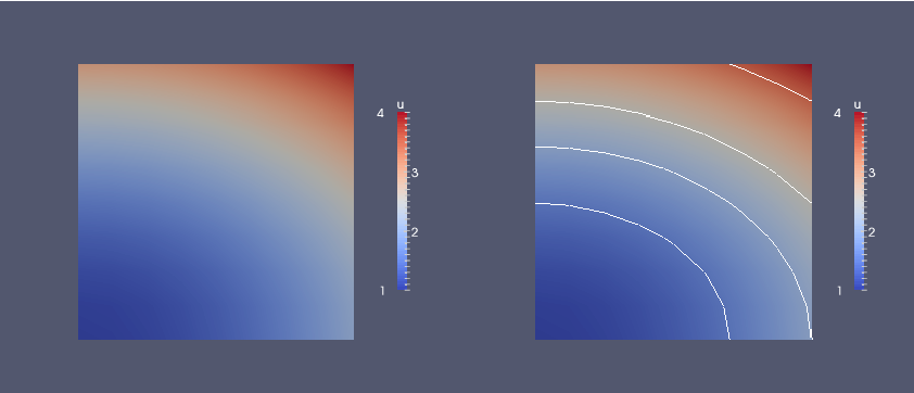
Visualization of the solution of the test problem in ParaView, with contour lines added in the right plot
Finally, we compute the error to check the accuracy of the solution.
We do this by comparing the finite element solution u with the exact
solution u_D, which in this example happens to be the same as the
Expression used to set the boundary conditions. We compute the error
in two different ways. First, we compute the \(L^2\) norm of the error,
defined by
Since the exact solution is quadratic and the finite element solution is piecewise linear, this error will be nonzero. To compute this error in FEniCS, we simply write
error_L2 = errornorm(u_D, u, 'L2')
The errornorm() function can also compute other error norms such
as the \(H^1\) norm. Type pydoc fenics.errornorm in a terminal window
for details.
We also compute the maximum value of the error at all the vertices of
the finite element mesh. As mentioned above, we expect this error to
be zero to within machine precision for this particular example. To
compute the error at the vertices, we first ask FEniCS to compute the
value of both u_D and u at all vertices, and then subtract the
results:
vertex_values_u_D = u_D.compute_vertex_values(mesh)
vertex_values_u = u.compute_vertex_values(mesh)
import numpy as np
error_max = np.max(np.abs(vertex_values_u_D - vertex_values_u))
We have here used the maximum and absolute value functions from numpy,
because these are much more efficient for large arrays (a factor of 30)
than Python’s built-n max and abs functions.
How to check that the error vanishes
With inexact arithmetics, as we always have on a computer, the maximum error at the vertices is not zero, but should be a small number. The machine precision is about \(10^{-16}\), but in finite element calculations, rounding errors of this size may accumulate, to produce an error larger than \(10^{-16}\). Experiments show that increasing the number of elements and increasing the degree of the finite element polynomials increases the error. For a mesh with \(2\times(20\times 20)\) cubic Lagrange elements (degree 3) the error is about \(2\cdot 10^{-12}\), while for 81 linear elements the error is about \(2\cdot 10^{-15}\).
A finite element function like \(u\) is expressed as a linear combination of basis functions \(\phi_j\), spanning the space \(V\):
By writing solve(a == L, u, bc) in the program, a linear system will
be formed from \(a\) and \(L\), and this system is solved for the
values \(U_1,\ldots,U_N\). The values \(U_1,\ldots,U_N\) are known as the
degrees of freedom (“dofs”) or nodal values of \(u\). For Lagrange
elements (and many other element types) \(U_j\) is simply the value of
\(u\) at the node with global number \(j\). The locations of the nodes and
cell vertices coincide for linear Lagrange elements, while for
higher-order elements there are additional nodes associated with the
facets, edges and sometimes also the interior of cells.
Having u represented as a Function object, we can either evaluate
u(x) at any point x in the mesh (expensive operation!), or we can
grab all the degrees of freedom in the vector \(U\) directly by
nodal_values_u = u.vector()
The result is a Vector object, which is basically an encapsulation
of the vector object used in the linear algebra package that is used
to solve the linear system arising from the variational problem.
Since we program in Python it is convenient to convert the Vector
object to a standard numpy array for further processing:
array_u = nodal_values_u.array()
With numpy arrays we can write MATLAB-like code to analyze the
data. Indexing is done with square brackets: array_u[j], where the
index j always starts at 0. If the solution is computed with
piecewise linear Lagrange elements (\(\mathsf{P}_1\)), then the size of
the array array_u is equal to the number of vertices, and each
array_u[j] is the value at some vertex in the mesh. However, the degrees
of freedom are not necessarily numbered in the same way as the
vertices of the
mesh, see the section Examining the degrees of freedom for details.
If we therefore want to know the values at the vertices, we need to
call the function u.compute_vertex_values(). This function returns
the values at all the vertices of the mesh as a numpy array with the same
numbering as for the vertices of the mesh, for example:
vertex_values_u = u.compute_vertex_values()
Note that for \(\mathsf{P}_1\) elements the arrays array_u and vertex_values_u have the same lengths and contain the same values, albeit in different order.
Our first FEniCS program for the Poisson equation targeted a simple test problem where we could easily verify the implementation. Now we turn the attention to a more physically relevant problem, in a non-trivial geometry, and that results in solutions of somewhat more exciting shape.
We want to compute the deflection \(D(x,y)\) of a two-dimensional, circular membrane, subject to a load \(p\) over the membrane. The appropriate PDE model is
Here, \(T\) is the tension in the membrane (constant), and \(p\) is the external pressure load. The boundary of the membrane has no deflection, implying \(D=0\) as boundary condition. A localized load can be modeled as a Gaussian function:
The parameter \(A\) is the amplitude of the pressure, \((x_0,y_0)\) the localization of the maximum point of the load, and \(\sigma\) the “width” of \(p\).
The localization of the pressure, \((x_0,y_0)\), is for simplicity set to \((0, R_0)\). There are many physical parameters in this problem, and we can benefit from grouping them by means of scaling. Let us introduce dimensionless coordinates \(\bar x = x/R\), \(\bar y = y/R\), and a dimensionless deflection \(w=D/D_c\), where \(D_c\) is a characteristic size of the deflection. Introducing \(\bar R_0=R_0/R\), we get
where
With an appropriate scaling, \(w\) and its derivatives are of size unity, so the left-hand side of the scaled PDE is about unity in size, while the right-hand side has \(\alpha\) as its characteristic size. This suggest choosing \(\alpha\) to be unity, or around unit. We shall in this particular case choose \(\alpha=4\). With this value, the solution is \(w(\bar x,\bar y) = 1-\bar x^2 - \bar y^2\). (One can also find the analytical solution in scaled coordinates and show that the maximum deflection \(D(0,0)\) is \(D_c\) if we choose \(\alpha=4\) to determine \(D_c\).) With \(D_c=AR^2/(8\pi\sigma T)\) and dropping the bars we get the scaled problem
to be solved over the unit circle with \(w=0\) on the boundary. Now there are only two parameters to vary: the dimensionless extent of the pressure, \(\beta\), and the localization of the pressure peak, \(R_0\in [0,1]\). As \(\beta\rightarrow 0\), we have a special case with solution \(w=1-x^2-y^2\).
Given a computed scaled solution \(w\), the physical deflection can be computed by
Just a few modifications are necessary in our previous program to solve this new problem.
A mesh over the unit circle can be created by the mshr tool in
FEniCS:
from mshr import *
domain = Circle(Point(0.0, 0.0), 1.0)
n = 20
mesh = generate_mesh(domain, n)
plot(mesh, interactive=True)
The Circle shape from mshr takes the center and radius of the circle
as the two first arguments, while n is the resolution, here the
suggested number of cells per radius.
The right-hand side pressure function
is represented by an Expression object. There
are two physical parameters in the formula for \(f\) that enter the
expression string and these parameters must have their values set
by keyword arguments:
beta = 8
R0 = 0.6
p = Expression(
    '4*exp(-pow(beta,2)*(pow(x[0], 2) + pow(x[1]-R0, 2)))',
    beta=beta, R0=R0)
The coordinates in Expression objects must be a vector
with indices 0, 1, and 2, and with the name x. Otherwise
we are free to introduce names of parameters as long as these are
given default values by keyword arguments. All the parameters
initialized by keyword arguments can at any time have their
values modified. For example, we may set
p.beta = 12
p.R0 = 0.3
We may introduce w instead of u as primary unknown and p instead
of f as right-hand side function:
w = TrialFunction(V)
v = TestFunction(V)
a = dot(grad(w), grad(v))*dx
L = p*v*dx

w = Function(V)
solve(a == L, w, bc)
It is of interest to visualize the pressure \(p\) along with the
deflection \(w\) so that we can examine membrane’s response to the
pressure. We must then transform the formula (Expression) to a
finite element function (Function). The most natural approach is to
construct a finite element function whose degrees of freedom are
calculated from \(p\). That is, we interpolate \(p\):
p = interpolate(p, V)
Note that the assignment to p destroys the previous Expression
object p, so if it is of interest to still have access to this
object, another name must be used for the Function object returned
by interpolate.
We can now plot w and p on the screen
as well as save the fields to file in VTK format:
plot(w, title='Deflection')
plot(p, title='Load')

vtkfile_w = File('membrane_deflection.pvd')
vtkfile_w << w
vtkfile_p = File('membrane_load.pvd')
vtkfile_p << p
Figure Load (left) and resulting deflection (right) of a circular membrane shows the result of the plot commands.
Load (left) and resulting deflection (right) of a circular membrane
The best way to compare the load and the deflection is to make a curve plot
along the line \(x=0\). This is just a matter of defining a set of points
along the line and evaluating the finite element functions w and p
at these points:
# Curve plot along x = 0 comparing p and w
import numpy as np
import matplotlib.pyplot as plt
tol = 1E-8  # avoid hitting points outside the domain
y = np.linspace(-1+tol, 1-tol, 101)
points = [(0, y_) for y_ in y]  # 2D points
w_line = np.array([w(point) for point in points])
p_line = np.array([p(point) for point in points])
plt.plot(y, 100*w_line, 'r-', y, p_line, 'b--') # magnify w
plt.legend(['100 x deflection', 'load'], loc='upper left')
plt.xlabel('y'); plt.ylabel('$p$ and $100u$')
plt.savefig('plot.pdf'); plt.savefig('plot.png')

# Hold plots
interactive()
plt.show()
The complete code can be found in the file ft02_poisson_membrane.py.
The resulting curve plot appears in Figure Comparison of membrane load and deflection. It is seen how the localized input (\(p\)) is heavily damped and smoothened in the output (\(w\)). This reflects a typical property of the Poisson equation.
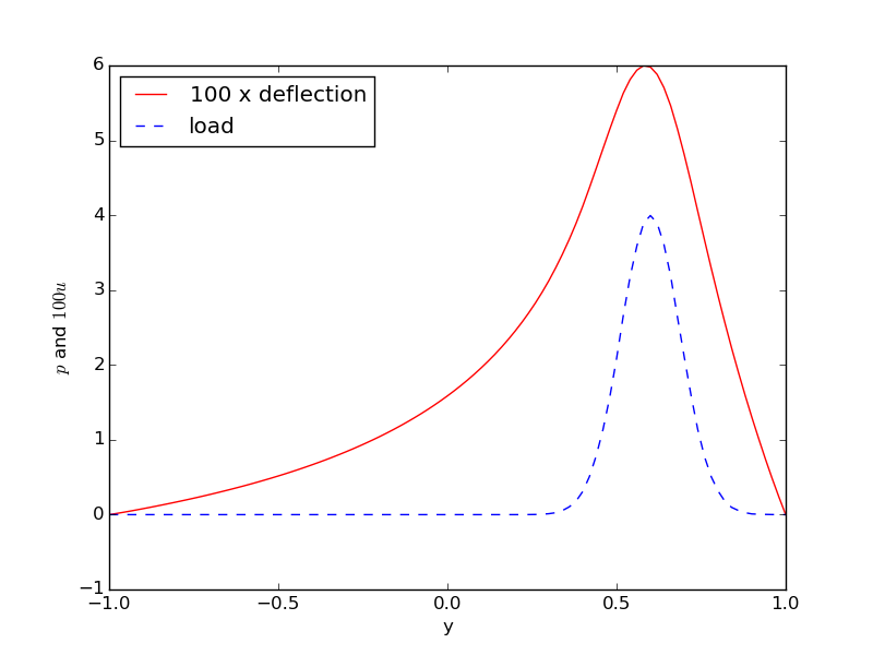
Comparison of membrane load and deflection
ParaView is a powerful tool for visualizing scalar and vector fields, including those computed by FEniCS.
Our program writes the fields \(w\) and \(p\) to file as finite element
functions. We choose the names of these files to be
membrane_deflection.pvd for \(w\) and membrane_load.pvd for \(p\).
These files are in VTK format and their data can be visualized in
ParaView. We now give a detailed account for how to visualize
the fields \(w\) and \(p\) in ParaView.
.pvd and
.vtu files. More specifically you will see membrane_deflection.pvd.
Choose this file.as surface, then load \(w\) again and plot as wireframe. Make sure both icons in the Pipeline Browser in the left part of the GUI are on for themembrane_deflection.pvdfiles you want to display. See Figure Default visualizations in ParaView: deflection (left, middle) and pressure load (right) (left).
Press the semi-sphere icon in the third row of buttons at the top of the GUI (the so-called filters). A set of contour values can now be specified at in a dialog box in the left part of the GUI. Remove the default contour (0.578808) and add 0.01, 0.02, 0.03, 0.04, 0.05. Click Apply and see an overlay of white contour lines. In the Pipeline Browser you can click on the icons to turn a filter on or off.
small icon. Choose the 3D View button. Open a new file and loadmembrane_load.pvd. Click on Apply to see a plot of the load.
click Apply to plot it, then select from the Filters pulldown menu the filter Warp By Scalar, click Apply, then toggle the 2D button to 3D in the Layout#1window (upper row of buttons in that window). Now you can rotate the figure. The height of the surface is very low, so go to the Properties (Warp By Scalar1) window to the left in the GUI and give a Scale Factor of 20 and re-click Apply to lift the surface by a factor of 20. Figure Default visualizations in ParaView: deflection (left, middle) and pressure load (right) (right) shows the result.
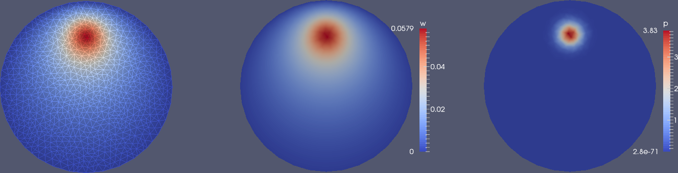
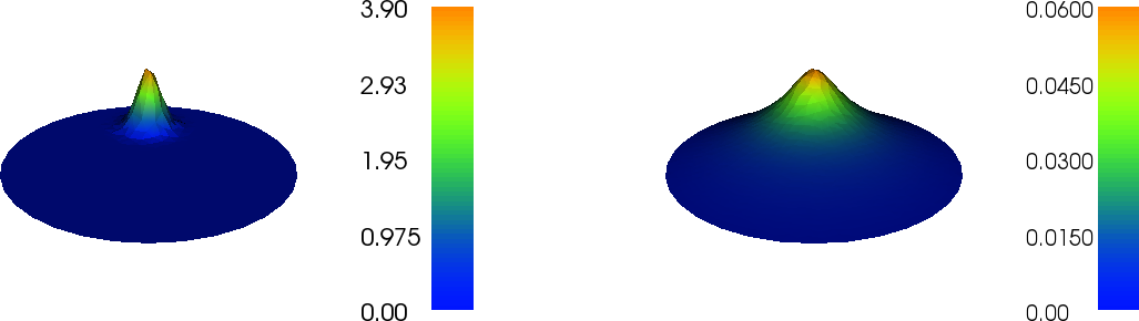
Default visualizations in ParaView: deflection (left, middle) and pressure load (right)
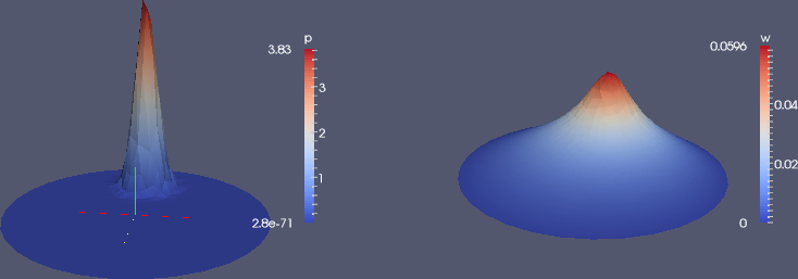
Use of Warp By Scalar filter to create lifted surfaces (with different vertical scales!) in ParaView: load (left) and deflection (right)
A particularly useful feature of ParaView is that you can record GUI clicks (Tools - Start/Stop Trace) and get them translated to Python code. This allows you automate the visualization process. You can also make curve plots along lines through the domain, etc.
For more information, we refer to The ParaView Guide [Ref24] (free PDF available) and to the ParaView tutorial as well as an instruction video.
This section explains some useful visualization features of the
built-in visualization tool in FEniCS. The plot command applies the
VTK package to visualize finite element functions in a very quick and
simple way. The command is ideal for debugging, teaching, and initial
scientific investigations. The visualization can be interactive, or
you can steer and automate it through program statements. More
advanced and professional visualizations are usually better created
with advanced tools like Mayavi, ParaView, or VisIt.
The plot function can take additional arguments, such as
a title of the plot, or a specification of a wireframe plot (elevated mesh)
instead of a colored surface plot:
plot(mesh, title='Finite element mesh')
plot(w, wireframe=True, title='Solution')
Axes can be turned on by the axes=True argument, while
interactive=True makes the program hang at the plot command - you have
to type q in the plot window to terminate the plot and continue execution.
The left mouse button is used to rotate the surface, while the right
button can zoom the image in and out. Point the mouse to the Help
text down in the lower left corner to get a list of all the keyboard
commands that are available.
The plots created by pressing p or P are stored in filenames
having the form dolfin_plot_X.png or dolfin_plot_X.pdf, where X
is an integer that is increased by one from the last plot that was
made. The file stem dolfin_plot_ can be set to something more
suitable through the hardcopy_prefix keyword argument to the plot
function, for instance, plot(f, hardcopy_prefix='pressure').
The ranges of the color scale can be set by the range_min and range_max
keyword arguments to plot. The values must be float objects. These
arguments are important to keep fixed for animations in time-dependent
problems.
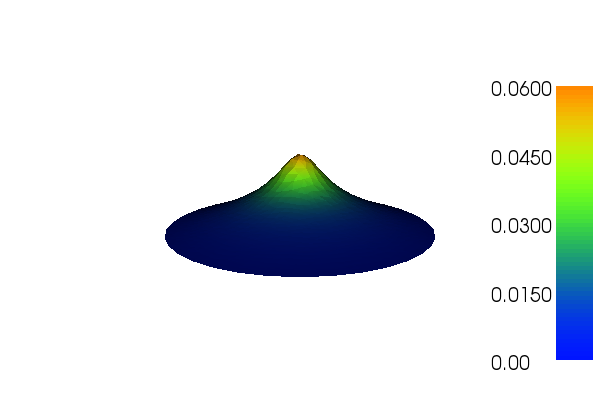
Plot of the deflection of a membrane using the built-in visualization tool
Built-in plotting on Mac OS X and in Docker
The built-in plotting in FEniCS may not work as expected when either
running on Mac OS X or when running inside a FEniCS Docker container.
FEniCS supports plotting using the plot() command on Mac OS
X. However, the keyboard shortcuts h, p, P and so on may fail
to work. When running inside a Docker container, plotting is not
supported since Docker does not interact with your windowing system.
For Docker users who need plotting, it is recommended to either work
within a Jupyter/FEniCS notebook (command fenicsproject notebook)
or rely on Paraview or other external tools for visualization.
[hpl 2: The solution refers to a solver function. This is not introduced before later, so present both a flat program and a solver function (as a teaser).]
Solve the problem \(-\nabla^2 u = f\) on the unit cube \([0,1]\times[0,1]\times [0,1]\) with \(u_0 = 1 + x^2 + 2y^2 - 4z^2\) on the boundary. Visualize the solution. Explore both the built-in visualization tool and ParaView.
Solution.
As hinted by the filename in this exercise,
a good starting point is the solver function in
the program ft03_poisson_function.py, which solves the corresponding 2D
problem. Only two lines in the body of solver needs to be changed (!):
mesh = .... Replace this line with
mesh = UnitCubeMesh(Nx, Ny, Nz)
and add Nz as argument to solver. We implement the new \(u_0\) function
in application_test and realize that the proper \(f(x,y,z)\) function
in this new case is 2.
u0 = Expression('1 + x[0]*x[0] + 2*x[1]*x[1] - 4*x[2]*x[2]')
f = Constant(2.0)
u = solver(f, u0, 6, 4, 3, 1)
The numerical solution is without approximation errors so we can
reuse the unit test from 2D, but it needs an extra Nz parameter.
The variation in \(u\) is only quadratic so a coarse mesh is okay for visualization. Below is plot from the ParaView (left) and the built-in visualization tool (right). The usage is as in 2D, but now one can use the mouse to rotate the 3D cube.
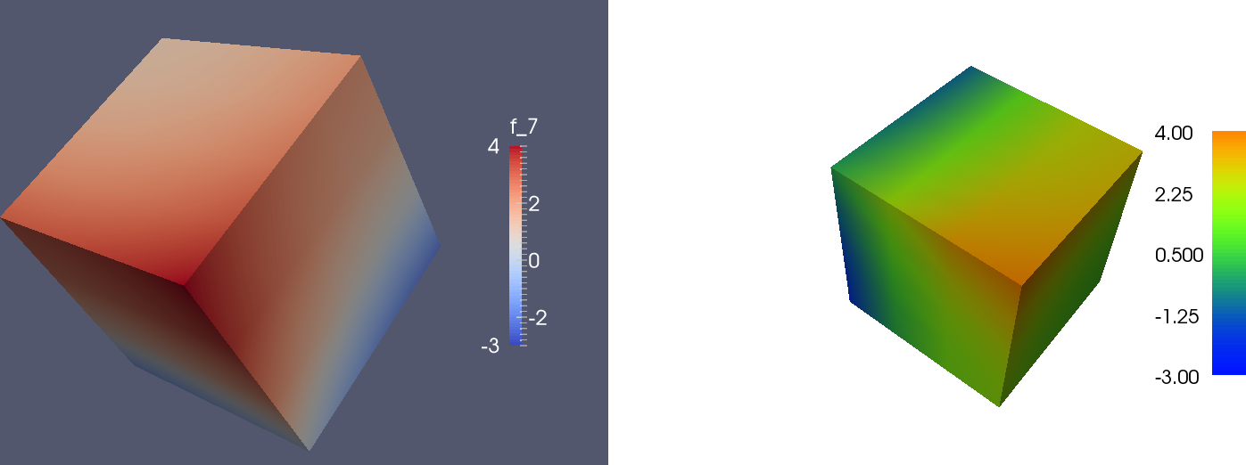
We can in ParaView add a contour filter and define contour surfaces for \(u=-2,1,0,1,2,3\), then add a slice filter to get a slice with colors:
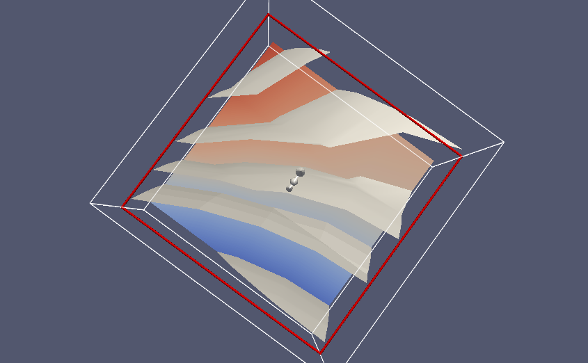
Filename: poissin_3d_func.