Make a web application that reads two numbers from a web page,
adds the numbers, and prints the sum in a new web page.
Package the necessary files that constitute the application
in a tar file.
Filename: add2.tar.gz.
Suppose you have tabular data in a file:
#  t        y       error
0.0000    1.2345   1.4E-4
1.0000    0.9871  -4.9E-3
1.2300    0.5545   8.2E-3
y and error should be plotted against
t, yielding two curves.
The web application may have one field: the name of the file to upload.
Search for constructions on how to upload a files and write this
application. Generate a suitable data file for testing purposes.
Filename: upload.tar.gz.
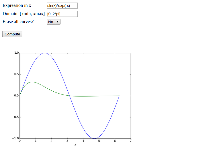
The purpose of this exercise is to write a web application that can visualize any user-given formula. For example, in the interface below,
the user has
sin(x)) to be plotted[0, 2*pi])sin(x)*exp(-x))
Hint 1.
You may use the vib1 app from the section Programming the Flask application
with the view_errcheck.html template as starting point.
Preferably, let plots be created as strings, as explained for the vib2
app in the section Avoiding plot files.
The Formula and Domain fields need to be TextField objects,
and the compute function must perform an eval on the user's input.
The Erase field is a SelectField object with selections Yes and
No. The former means that the compute function calls the figure
function in Matplotlib before creating a new plot. If this is not
done, a new formula will be plotting in the same figure as the last one.
With the Yes/No selection, it is possible either plot individual curves
or compare curves in the same plot.
Hint 2.
Performing eval on the user's input requires that names like
sin, exp, and pi are defined. The simplest approach is to
do a
from numpy import *
numpy are then available as global variables and one can simply
do domain = eval(domain) to turn the string domain coming from
the Domain text field into a Python list with two elements.
A better approach is not to rely on global variables, but run eval
in the numpy namespace:
import numpy
domain = eval(domain, numpy.__dict__)
The evaluation of the formula is slightly more complicated if eval
is to be run with the numpy namespace. One first needs
to create \( x \) coordinates:
x = numpy.linspace(domain[0], domain[1], 10001)
eval(formula, numpy.__dict__) will not work because a formula
like sin(x) needs both sin and x in the namespace. The latter
is not in the namespace and must be explicitly included. A new namespace
can be made:
namespace = numpy.__dict__.copy()
namespace.update({'x': x})
formula = eval(formula, namespace)
Hint 3. You should add tests when evaluating and using the strings from input as these may have wrong syntax.
Filename: plot_formula.tar.gz.
This exercise develops a web application that can plot Taylor polynomial approximations of any degree to any user-given formula. You should do Exercise 3: Plot a user-specified formula first as many of the techniques there must be used and even further developed in the present exercise.
The figure below shows an example of what one can do in the web app:
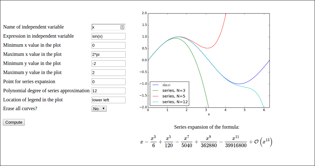
Here, the user has
sin(x))sympy to produce Taylor polynomial expansions of arbitrary
expressions. Here is a session demonstrating how to obtain the
series expansion of \( e^{-x}\sin (\pi x) \) to 2nd degree.
>>> import sympy as sp
>>> x = sp.symbols('x')
>>> f = sp.exp(-x)*sp.sin(sp.pi*x)
>>> f.series(x, 0, 3)
pi*x - pi*x**2 + O(x**3)
>>> sp.latex(f.series(x, 0, 3))
'\\pi x - \\pi x^{2} + \\mathcal{O}\\left(x^{3}\\right)'
>>> fs = f.series(x, 0, 3).removeO()  # get rid of O() term
>>> fs
-pi*x**2 + pi*x
>>> f_func = sp.lambdify([x], fs)     # make Python function
>>> f_func(1)
0.0
>>> f_func(2)
-6.283185307179586
Basically, the steps above must be carried out to create a Python
function for the series expansion such that it can be plotted.
A similar sp.lambdify call on the original formula is also necessary
to plot that one.
However, the challenge is that the formula is available only as a
string, and it may contain an independent variable whose name is also
only available through a string from the web interface. That is, we
may give formulas like exp(-t) if t is chosen as independent
variable. Also, the expression does not contain function names
prefixed with sympy or sp, just plain names like sin, cos,
exp, etc. An example on formula is cos(pi*x) + log(x).
a) Write a function
def formula2series2pyfunc(formula, N, x, x0=0):
sympy formula, and integer N, a sympy symbol x
and another sympy symbol x0 and returns
1) a Python function for formula, 2) a Python function for the
series expansion of degree N of the formula around x0, and
3) a LaTeX string containing the formula for the series expansion.
Put the function in a file compute.py. You should thereafter be able to run
the following session:
>>> import compute
>>> import sympy as sp
>>> from sympy import *
>>> t = symbols('t')
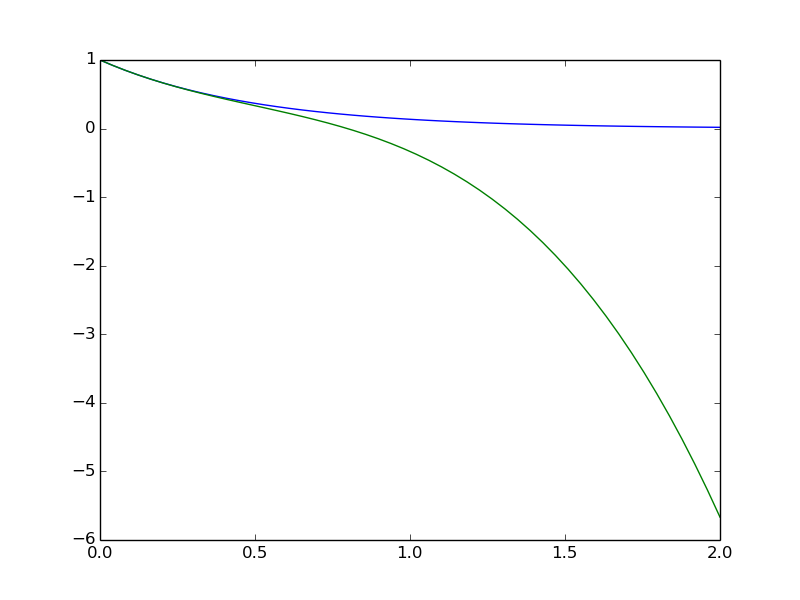
>>> formula = exp(-2*t)
>>> f, s, latex = compute.formula2series2pyfunc(formula, 3, t)
>>> latex
'- \\frac{4 t^{3}}{3} + 2 t^{2} - 2 t + 1'
>>> import matplotlib.pyplot as plt
>>> import numpy as np
>>> t = np.linspace(0, 2)
>>> plt.plot(t, f(t), t, s(t))
[<matplotlib.lines.Line2D at 0x7fc6c020f350>,
<matplotlib.lines.Line2D at 0x7fc6c020f5d0>]
>>> plt.show()
Hint.
The series expansion is obtained by formula.series(x, x0, N),
but the output contains an O() term which makes it impossible to
convert the expression to a Python function via sympy.lambify.
Use
series = formula.series(x, x0, N+1).removeO()
sympy.lambdify.
We use N+1 since N in the series function refers to the degree
of the O() term, which is now removed.
For the LaTeX expression it is natural to have the O() term:
latex = sympy.latex(formula.series(x, x0, N+1))
removeO() is used).
b) Write the compute function:
def visualize_series(
    formula,                  # string: formula
    independent_variable,     # string: name of independent var.
    N,                        # int: degree of polynomial approx.
    xmin, xmax, ymin, ymax,   # strings: extent of axes
    legend_loc,               # string: upper left, etc.
    x0='0',                   # string: point of expansion
    erase='yes',              # string: 'yes' or 'no'
    ):
Hint 1.
Converting the string formula to a valid sympy expression is
challenging. First, create a local variable for a sympy symbol
with the content of
independent_variable as name, since such a variable is needed
with performing eval on formula. Also introduce a variable x
to point to the same sympy symbol. Relevant code is
# Turn independent variable into sympy symbol, stored in x
import sympy as sp
exec('x = %s = sp.symbols("%s")' %
     (independent_variable, independent_variable))
Hint 2.
Evaluating formula in the namespace of sympy (so that all the sin,
exp, pi, and similar symbols are defined properly as sympy
objects) needs a merge of the sympy namespace and the variable for
the sympy symbol representing the independent variable:
namespace = sp.__dict__.copy()
local = {}
local[independent_variable] = x
namespace.update(local)
formula = eval(formula, namespace)
x0 into a valid sympy expression is easier: x0 = eval(x0, sp.__dict__).
Hint 3.
Note that in the web interface, the minimum and maximum values on the axis
can be mathematical expressions such as 2*pi. This means that these
quantities must be strings that are evaluated in the numpy namespace, e.g.,
import numpy as np
xmin = eval(xmin, np.__dict__)
Hint 4.
Getting the legends right when plotting multiple curves in the same
plot is a bit tricky. One solution is to have a global variable legends
that is initialized to [] and do the following inside the compute function:
import matplotlib.pyplot as plt
global legends
if erase == 'yes':   # Start new figure?
    plt.figure()
    legends = []
if not legends:
    # We come here every time the figure is empty so
    # we need to draw the formula
    legends.append('$%s$' % sp.latex(formula))
    plt.plot(x, f(x))
f is the Python function for computing the numpy variant
of the expression in formula.
Hint 5.
Use the test block in the file to call the compute function several
times with different values of the erase parameter to test that
the erase functionality is correct.
c) Write the remaining files. These have straightforward content if Exercise 3: Plot a user-specified formula is done and understood.
Filename: Taylor_approx.tar.gz.
gen app
Add a new argument x_axis to the compute function in the
gen
application from the section Autogenerating the code. The x_axis argument measures the extent
of the \( x \) axis in the plots in terms of the number of standard
deviations (default may be 7). Observe how the web interface
automatically adds the new argument and how the plots adapt!
The purpose of this exercise is to look into web apps with multipe submit buttons. More precisely, we want a web app that can perform two actions: add \( a+b \) and multiply \( pq \). There should be two parts of the open web page:
Add button. Clicking on Add
brings up a new line below add: Sum: 3 if \( a+b=3 \).Multiply button. Clicking on Multiply
brings up a new line below add: Product: 5 if \( pq=5 \).
Hint 1.
Make two input form classes, say AddForm and MulForm in model.py.
Since it suffices to fill in either \( a \) and \( b \) or \( p \) and \( q \), all
fields cannot be required.
Let the controller process both classes and collect the two forms
and two results in a form dictionary and a result dictionary
that is passed on the to the view.html file.
Hint 2.
To detect which "subapp" (add or multply) that was used, one can
give a name to the submit button and in the controller check which
of the submit buttons that was pressed (and then perform the associated
computation and update of results). In view.html:
<input type="submit" name="btn" value="Add"></form>
...
<input type="submit" name="btn" value="Multiply"></form>
controller.py:
if request.method == 'POST' and f.validate() and \
       request.form['btn'] == 'Multiply':
    result['mul'] = mul(f.p.data, f.q.data)
Filename: addmul.tar.gz.
gen app with more data types
In the gen
application from the section Autogenerating the code,
use the label argument in the form field objects to add an
information of the type of data that is to be supplied in the
text field. Extend the model.py file to also handle
lists, tuples, and Numerical Python arrays. For these three
new data types, use a TextField object and run eval
on the text in the view.py file.
A simple test is to extend the compute function with an
argument x_range for the range of the \( x \) axis, specified as
an interval (2-list or 2-tuple).
Filename: gen_ext.tar.gz.
Given a compute with a set of positional and keyword
arguments, the purpose of this exercise is to automatically generate the
Flask files model.py and controller.py. Use the Python inspect
module, see the section Autogenerating the code, to extract
the positional and keyword arguments in compute, and use this
information to construct the relevant Python code in strings. Write
the strings to model.py and controller.py files. Assume as
in the section Autogenerating the code that the user provides
a file view_results.html for defining how the returned object
from the compute function is to be rendered.
Test the code generator on the compute function in the vib1
application to check that the generated
model.py and controller.py files are correct.
Filename: generate_flask.py.
The Bokeh Python library works very well with Flask. The purpose of this exercise is to make a web app where one can explore how parameters in a function influence the function's shape. Given some function \( f(x;p_0,p_1,\ldots,p_n) \), where \( x \) is the independent variable and \( p_0,p_1,\ldots,p_n \) are parameters, we want to create a user interface with a plot field and text fields or sliders for \( p_0,p_1,\ldots,p_n \) such that altering any parameter immediately updates the graph of the \( f \) as a function of \( x \). The Bokeh web side contains a demo: for the specific function $$ f(x;x_0,A,\phi,\omega)= x_0 + A\sin(\omega (x + \phi)).$$ However, this project is about accepting any function \( f(x;p_0,p_1,\ldots,p_n) \) and creating tailored Flask/Bokeh code of the type in the demo. The user must specify a Python function for \( f \):
def f(x, p):
    x_0, A, phi, omega = p
    return x_0 + A*sin(omega*(x - phi))
p is a list of parameter values. In addition, the user must
provide info about each parameter: the name, a range or a number,
and if range, a default value. Here is an example:
p_info = [
    ('offset', [-2, 2], 0),
    ('amplitude', [0, 5], 2.5),
    ('phase', 0),
    ('frequency', [1, 10], 1)]
phase in this example,
get a text field where the user can alter the number.
The user must also provide a suitable range for the \( x \) axis. As test case beyond the example above, try a Gaussian function with this input from the user:
import numpy as np

def gaussian(x, p):
    mu, sigma = p
    return 1./(sigma*np.sqrt(2*np.pi))*\
           np.exp(-0.5*(x - mu)**2/sigma**2)

p_info = [
    ('mean', [-2, 2], 0),
    ('standard deviation', [0.1, 4], 1)]

x_axis = [-10, 10]
expore_func.tar.gz.
numpy, scipy, or matplotlib)