Solving partial differential equations

The subject of partial differential equations (PDEs) is enormous. At the same time, it is very important, since so many phenomena in nature and technology find their mathematical formulation through such equations. Knowing how to solve at least some PDEs is therefore of great importance to engineers. In an introductory book like this, nowhere near full justice to the subject can be made. However, we still find it valuable to give the reader a glimpse of the topic by presenting a few basic and general methods that we will apply to a very common type of PDE.

We shall focus on one of the most widely encountered partial differential equations: the diffusion equation, which in one dimension looks like

\[\frac{\partial u}{\partial t} = \beta\frac{\partial^2 u}{\partial x^2} + g \thinspace .\]

The multi-dimensional counterpart is often written as

\[\frac{\partial u}{\partial t} = \beta\nabla^2 u + g \thinspace .\]

We shall restrict the attention here to the one-dimensional case.

The unknown in the diffusion equation is a function \(u(x,t)\) of space and time. The physical significance of \(u\) depends on what type of process that is described by the diffusion equation. For example, \(u\) is the concentration of a substance if the diffusion equation models transport of this substance by diffusion. Diffusion processes are of particular relevance at the microscopic level in biology, e.g., diffusive transport of certain ion types in a cell caused by molecular collisions. There is also diffusion of atoms in a solid, for instance, and diffusion of ink in a glass of water.

One very popular application of the diffusion equation is for heat transport in solid bodies. Then \(u\) is the temperature, and the equation predicts how the temperature evolves in space and time within the solid body. For such applications, the equations is known as the heat equation. We remark that the temperature in a fluid is influenced not only by diffusion, but also by the flow of the liquid. If present, the latter effect requires an extra term in the equation (known as an advection or convection term).

The term \(g\) is known as the source term and represents generation, or loss, of heat (by some mechanism) within the body. For diffusive transport, \(g\) models injection or extraction of the substance.

We should also mention that the diffusion equation may appear after simplifying more complicated partial differential equations. For example, flow of a viscous fluid between two flat and parallel plates is described by a one-dimensional diffusion equation, where \(u\) then is the fluid velocity.

A partial differential equation is solved in some domain \(\Omega\) in space and for a time interval \([0,T]\). The solution of the equation is not unique unless we also prescribe initial and boundary conditions. The type and number of such conditions depend on the type of equation. For the diffusion equation, we need one initial condition, \(u(x,0)\), stating what \(u\) is when the process starts. In addition, the diffusion equation needs one boundary condition at each point of the boundary \(\partial\Omega\) of \(\Omega\). This condition can either be that \(u\) is known or that we know the normal derivative, \(\nabla u\cdot\boldsymbol{n}=\partial u/ \partial n\) (\(\boldsymbol{n}\) denotes an outward unit normal to \(\partial\Omega\)).

Let us look at a specific application and how the diffusion equation with initial and boundary conditions then appears. We consider the evolution of temperature in a one-dimensional medium, more precisely a long rod, where the surface of the rod is covered by an insulating material. The heat can then not escape from the surface, which means that the temperature distribution will only depend on a coordinate along the rod, \(x\), and time \(t\). At one end of the rod, \(x=L\), we also assume that the surface is insulated, but at the other end, \(x=0\), we assume that we have some device for controlling the temperature of the medium. Here, a function \(s(t)\) tells what the temperature is in time. We therefore have a boundary condition \(u(0,t)=s(t)\). At the other insulated end, \(x=L\), heat cannot escape, which is expressed by the boundary condition \(\partial u(L,t)/\partial x=0\). The surface along the rod is also insulated and hence subject to the same boundary condition (here generalized to \(\partial u/\partial n=0\) at the curved surface). However, since we have reduced the problem to one dimension, we do not need this physical boundary condition in our mathematical model. In one dimension, we can set \(\Omega = [0,L]\).

To summarize, the partial differential equation with initial and boundary conditions reads

\[\tag{120} \frac{\partial u(x,t)}{\partial t} = \beta \frac{\partial^{2}u(x,t)}{\partial x^2} + g(x,t), x \in \left(0,L\right), t \in (0,T],\]

\[\tag{121} u(0,t) = s(t), t \in (0,T],\]

\[\tag{122} \frac{\partial}{\partial x}u(L,t) = 0, t \in (0,T],\]

\[\tag{123} u(x,0) = I(x), x \in \left[0,L\right]\]\[ \thinspace .\]

Mathematically, we assume that at \(t=0\), the initial condition (123) holds and that the partial differential equation (120) comes into play for \(t>0\). Similarly, at the end points, the boundary conditions (121) and (122) govern \(u\) and the equation therefore is valid for \(x\in (0,L)\).

Boundary and initial conditions are needed

The initial and boundary conditions are extremely important. Without them, the solution is not unique, and no numerical method will work. Unfortunately, many physical applications have one or more initial or boundary conditions as unknowns. Such situations can be dealt with if we have measurements of \(u\), but the mathematical framework is much more complicated.

What about the source term \(g\) in our example with temperature distribution in a rod? \(g(x,t)\) models heat generation inside the rod. One could think of chemical reactions at a microscopic level in some materials as a reason to include \(g\). However, in most applications with temperature evolution, \(g\) is zero and heat generation usually takes place at the boundary (as in our example with \(u(0,t)=s(t)\)).

Before continuing, we may consider an example of how the temperature distribution evolves in the rod. At time \(t=0\), we assume that the temperature is \(10^{\circ}\) C. Then we suddenly apply a device at \(x=0\) that keeps the temperature at \(50^{\circ}\) C at this end. What happens inside the rod? Intuitively, you think that the heat generation at the end will warm up the material in the vicinity of \(x=0\), and as time goes by, more and more of the rod will be heated, before the entire rod has a temperature of \(50^{\circ}\) C (recall that no heat escapes from the surface of the rod).

Mathematically, (with the temperature in Kelvin) this example has \(I(x)=283\) K, except at the end point: \(I(0)=323\) K, \(s(t) = 323\) K, and \(g=0\). The figure below shows snapshots from four different times in the evolution of the temperature.

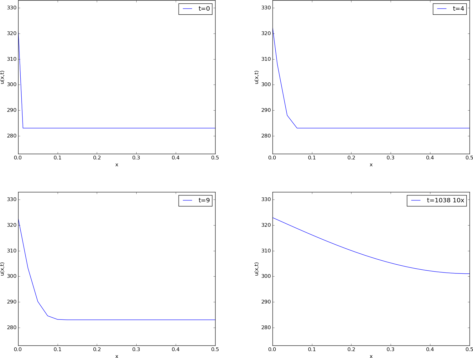
Snapshots of temperature distribution.

Finite difference methods

We shall now construct a numerical method for the diffusion equation. We know how to solve ordinary differential equations, so in a way we are able to deal with the time derivative. Very often in mathematics, a new problem can be solved by reducing it to a series of problems we know how to solve. In the present case, it means that we must do something with the spatial derivative \(\partial^2 /\partial x^2\) in order to reduce the partial differential equation to ordinary differential equations. One important technique for achieving this, is based on finite difference discretization of spatial derivatives.

Reduction of a PDE to a system of ODEs

Introduce a spatial mesh in \(\Omega\) with mesh points

\[\begin{split}x_0=0 < x_1 < x_2 < \cdots < x_N=L \thinspace .\end{split}\]

The space between two mesh points \(x_i\) and \(x_{i+1}\), i.e. the interval \([x_i,x_{i+1}]\), is call a cell. We shall here, for simplicity, assume that each cell has the same length \(\Delta x = x_{i+1}-x_i\), \(i=0,\ldots, N-1\).

The partial differential equation is valid at all spatial points \(x\in\Omega\), but we may relax this condition and demand that it is fulfilled at the internal mesh points only, \(x_1,\ldots,x_{N-1}\):

\[\tag{124} \frac{\partial u(x_i,t)}{\partial t} = \beta \frac{\partial^{2}u(x_i,t)}{\partial x^2} + g(x_i,t),\quad i=1,\ldots,N-1 \thinspace .\]

Now, at any point \(x_i\) we can approximate the second-order derivative by a finite difference:

\[\tag{125} \frac{\partial^{2}u(x_i,t)}{\partial x^2} \approx \frac{u(x_{i+1},t) - 2u(x_i,t) + u(x_{i-1},t)}{\Delta x^2}\thinspace .\]

It is common to introduce a short notation \(u_i(t)\) for \(u(x_i,t)\), i.e., \(u\) approximated at some mesh point \(x_i\) in space. With this new notation we can, after inserting (125) in (124), write an approximation to the partial differential equation at mesh point \((x_i,t\)) as

\[\tag{126} \frac{d u_i(t)}{d t} = \beta \frac{u_{i+1}(t) - 2u_i(t) + u_{i-1}(t)}{\Delta x^2} + g_i(t),\quad i=1,\ldots,N-1 \thinspace .\]

Note that we have adopted the notation \(g_i(t)\) for \(g(x_i,t)\) too.

What is (126)? This is nothing but a system of ordinary differential equations in \(N-1\) unknowns \(u_1(t),\ldots,u_{N-1}(t)\)! In other words, with aid of the finite difference approximation (125), we have reduced the single partial differential equation to a system of ODEs, which we know how to solve. In the literature, this strategy is called the method of lines.

We need to look into the initial and boundary conditions as well. The initial condition \(u(x,0)=I(x)\) translates to an initial condition for every unknown function \(u_i(t)\): \(u_i(0)=I(x_i)\), \(i=0,\ldots,N\). At the boundary \(x=0\) we need an ODE in our ODE system, which must come from the boundary condition at this point. The boundary condition reads \(u(0,t)=s(t)\). We can derive an ODE from this equation by differentiating both sides: \(u_0'(t)=s'(t)\). The ODE system above cannot be used for \(u_0'\) since that equation involves some quantity \(u_{-1}'\) outside the domain. Instead, we use the equation \(u_0'(t)=s'(t)\) derived from the boundary condition. For this particular equation we also need to make sure the initial condition is \(u_0(0)=s(0)\) (otherwise nothing will happen: we get \(u=283\) K forever).

We remark that a separate ODE for the (known) boundary condition \(u_0=s(t)\) is not strictly needed. We can just work with the ODE system for \(u_1,\ldots,u_{N}\), and in the ODE for \(u_0\), replace \(u_0(t)\) by \(s(t)\). However, these authors prefer to have an ODE for every point value \(u_i\), \(i=0,\ldots,N\), which requires formulating the known boundary at \(x=0\) as an ODE. The reason for including the boundary values in the ODE system is that the solution of the system is then the complete solution at all mesh points, which is convenient, since special treatment of the boundary values is then avoided.

The condition \(\partial u/\partial x=0\) at \(x=L\) is a bit more complicated, but we can approximate the spatial derivative by a centered finite difference:

\[\left.\frac{\partial u}{\partial x}\right|_{i=N}\approx \frac{u_{N+1}-u_{N-1}}{2\Delta x} = 0\thinspace .\]

This approximation involves a fictitious point \(x_{N+1}\) outside the domain. A common trick is to use (126) for \(i=N\) and eliminate \(u_{N+1}\) by use of the discrete boundary condition (\(u_{N+1}=u_{N-1}\)):

\[\tag{127} \frac{d u_N(t)}{d t} = \beta \frac{2u_{N-1}(t) - 2u_N(t)}{\Delta x^2} + g_N(t)\thinspace .\]

That is, we have a special version of (126) at the boundary \(i=N\).

What about simpler finite differences at the boundary

Some reader may think that a smarter trick is to approximate the boundary condition \(\partial u/\partial x\) at \(x=L\) by a one-sided difference:

\[\left.\frac{\partial u}{\partial x}\right|_{i=N}\approx \frac{u_{N}-u_{N-1}}{\Delta x} = 0\thinspace .\]

This gives a simple equation \(u_N=u_{N-1}\) for the boundary value, and a corresponding ODE \(u_N'=u_{N-1}'\). However, this approximation has an error of order \(\Delta x\), while the centered approximation we used above has an error of order \(\Delta x^2\). The finite difference approximation we used for the second-order derivative in the diffusion equation also has an error of order \(\Delta x^2\). Thus, if we use the simpler one-sided difference above, it turns out that we reduce the overall accuracy of the method.

We are now in a position to summarize how we can approximate the partial differential equation problem (120)-(123) by a system of ordinary differential equations:

\[\tag{128} \frac{du_0}{dt} = s'(t),\]

\[\tag{129} \frac{du_i}{dt} = \frac{\beta}{\Delta x^2} (u_{i+1}(t) - 2u_i(t) + u_{i-1}(t)) + g_i(t),\quad i=1,\ldots,N-1,\]

\[\tag{130} \frac{du_N}{dt} = \frac{2\beta}{\Delta x^2} (u_{N-1}(t) - u_N(t)) + g_N(t)\thinspace .\]

The initial conditions are

\[\tag{131} u_0(0) = s(0),\]

\[\tag{132} u_i(0) = I(x_i),\quad i=1,\ldots,N\thinspace .\]

We can apply any method for systems of ODEs to solve (128)-(130).

Construction of a test problem with known discrete solution

At this point, it is tempting to implement a real physical case and run it. However, partial differential equations constitute a non-trivial topic where mathematical and programming mistakes come easy. A better start is therefore to address a carefully designed test example where we can check that the method works. The most attractive examples for testing implementations are those without approximation errors, because we know exactly what numbers the program should produce. It turns out that solutions \(u(x,t)\) that are linear in time and in space can be exactly reproduced by most numerical methods for partial differential equations. A candidate solution might be

\[u(x,t) = (3t+2)(x-L)\thinspace .\]

Inserting this \(u\) in the governing equation gives

\[3(x-L) = 0 + g(x,t) \quad\Rightarrow\quad g(x,t)= 3(x-L) \thinspace .\]

What about the boundary conditions? We realize that \(\partial u/\partial x = 3t+2\) for \(x=L\), which breaks the assumption of \(\partial u/\partial x=0\) at \(x=L\) in the formulation of the numerical method above. Moreover, \(u(0,t)=-L(3t+2)\), so we must set \(s(t)=-L(3t+2)\) and \(s'(t)=-3L\). Finally, the initial condition dictates \(I(x)=2(x-L)\), but recall that we must have \(u_0=s(0)\), and \(u_i=I(x_i)\), \(i=1,\ldots,N\): it is important that \(u_0\) starts out at the right value dictated by \(s(t)\) in case \(I(0)\) is not equal this value.

First we need to generalize our method to handle \(\partial u/\partial x=\gamma \neq 0\) at \(x=L\). We then have

\[\frac{u_{N+1}(t)- u_{N-1}(t)}{2\Delta x}= \gamma\quad\Rightarrow \quad u_{N+1} = u_{N-1} + 2\gamma \Delta x,\]

which inserted in (126) gives

\[\tag{133} \frac{d u_N(t)}{d t} = \beta \frac{2u_{N-1}(t) + 2\gamma\Delta x - 2u_N(t)}{\Delta x^2} + g_N(t)\thinspace .\]

Implementation: Forward Euler method

In particular, we may use the Forward Euler method as implemented in the general function ode_FE in the module ode_system_FE from the section Programming the numerical method; the general case. The ode_FE function needs a specification of the right-hand side of the ODE system. This is a matter of translating (128), (129), and (133) to Python code (in file test_diffusion_pde_exact_linear.py):

def rhs(u, t):
    N = len(u) - 1
    rhs = zeros(N+1)
    rhs[0] = dsdt(t)
    for i in range(1, N):
        rhs[i] = (beta/dx**2)*(u[i+1] - 2*u[i] + u[i-1]) + \
                 g(x[i], t)
    rhs[N] = (beta/dx**2)*(2*u[N-1] + 2*dx*dudx(t) -
                           2*u[N]) + g(x[N], t)
    return rhs

def u_exact(x, t):
    return (3*t + 2)*(x - L)

def dudx(t):
    return (3*t + 2)

def s(t):
    return u_exact(0, t)

def dsdt(t):
    return 3*(-L)

def g(x, t):
    return 3*(x-L)

Note that dudx(t) is the function representing the \(\gamma\) parameter in (133). Also note that the rhs function relies on access to global variables beta, dx, L, and x, and global functions dsdt, g, and dudx.

We expect the solution to be correct regardless of \(N\) and \(\Delta t\), so we can choose a small \(N\), \(N=4\), and \(\Delta t = 0.1\). A test function with \(N=4\) goes like

def test_diffusion_exact_linear():
    global beta, dx, L, x  # needed in rhs
    L = 1.5
    beta = 0.5
    N = 4
    x = linspace(0, L, N+1)
    dx = x[1] - x[0]
    u = zeros(N+1)

    U_0 = zeros(N+1)
    U_0[0] = s(0)
    U_0[1:] = u_exact(x[1:], 0)
    dt = 0.1
    print dt

    u, t = ode_FE(rhs, U_0, dt, T=1.2)

    tol = 1E-12
    for i in range(0, u.shape[0]):
        diff = abs(u_exact(x, t[i]) - u[i,:]).max()
        assert diff < tol, 'diff=%.16g' % diff
        print 'diff=%g at t=%g' % (diff, t[i])

With \(N=4\) we reproduce the linear solution exactly. This brings confidence to the implementation, which is just what we need for attacking a real physical problem next.

Problems with reusing the rhs function

The rhs function must take u and t as arguments, because that is required by the ode_FE function. What about the variables beta, dx, L, x, dsdt, g, and dudx that the rhs function needs? These are global in the solution we have presented so far. Unfortunately, this has an undesired side effect: we cannot import the rhs function in a new file, define dudx and dsdt in this new file and get the imported rhs to use these functions. The imported rhs will use the global variables, including functions, in its own module.

How can we find solutions to this problem? Technically, we must pack the extra data beta, dx, L, x, dsdt, g, and dudx with the rhs function, which requires more advanced programming considered beyond the scope of this text.

A class is the simplest construction for packing a function together with data, see the beginning of Chapter 7 in [Ref18] for a detailed example on how classes can be used in such a context. Another solution in Python, and especially in computer languages supporting functional programming, is so called closures. They are also covered in Chapter 7 in the mentioned reference and behave in a magic way. The third solution is to allow an arbitrary set of arguments for rhs in a list to be transferred to ode_FE and then back to rhs. Appendix H.4 in [Ref18] explains the technical details.

Application: heat conduction in a rod

Let us return to the case with heat conduction in a rod (120)-(123). Assume that the rod is 50 cm long and made of aluminum alloy 6082. The \(\beta\) parameter equals \(\kappa/(\varrho c)\), where \(\kappa\) is the heat conduction coefficient, \(\varrho\) is the density, and \(c\) is the heat capacity. We can find proper values for these physical quantities in the case of aluminum alloy 6082: \(\varrho = 2.7\cdot 10^3\hbox{ kg/m}^3\), \(\kappa = 200\,\,\frac{\hbox{W}}{\hbox{mK}}\), \(c=900\,\,\frac{\hbox{J}}{\hbox{Kkg}}\). This results in \(\beta = \kappa/(\varrho c) = 8.2\cdot 10^{-5}\hbox{ m}^2/\hbox{s}\). Preliminary simulations show that we are close to a constant steady state temperature after 1 h, i.e., \(T=3600\) s.

The rhs function from the previous section can be reused, only the functions s, dsdt, g, and dudx must be changed (see file rod_FE.py):

def dudx(t):
    return 0

def s(t):
    return 323

def dsdt(t):
    return 0

def g(x, t):
    return 0

Parameters can be set as

L = 0.5
beta = 8.2E-5
N = 40
x = linspace(0, L, N+1)
dx = x[1] - x[0]
u = zeros(N+1)

U_0 = zeros(N+1)
U_0[0] = s(0)
U_0[1:] = 283

Let us use \(\Delta t = 0.00034375\). We can now call ode_FE and then make an animation on the screen to see how \(u(x,t)\) develops in time:

t0 = time.clock()
from ode_system_FE import ode_FE
u, t = ode_FE(rhs, U_0, dt, T=1*60*60)
t1 = time.clock()
print 'CPU time: %.1fs' % (t1 - t0)

# Make movie
import os
os.system('rm tmp_*.png')
import matplotlib.pyplot as plt
plt.ion()
y = u[0,:]
lines = plt.plot(x, y)
plt.axis([x[0], x[-1], 273, s(0)+10])
plt.xlabel('x')
plt.ylabel('u(x,t)')
counter = 0
# Plot each of the first 100 frames, then increase speed by 10x
change_speed = 100
for i in range(0, u.shape[0]):
    print t[i]
    plot = True if i <= change_speed else i % 10 == 0
    lines[0].set_ydata(u[i,:])
    if i > change_speed:
        plt.legend(['t=%.0f 10x' % t[i]])
    else:
        plt.legend(['t=%.0f' % t[i]])
    plt.draw()
    if plot:
        plt.savefig('tmp_%04d.png' % counter)
        counter += 1
    #time.sleep(0.2)

The plotting statements update the \(u(x,t)\) curve on the screen. In addition, we save a fraction of the plots to files tmp_0000.png, tmp_0001.png, tmp_0002.png, and so on. These plots can be combined to ordinary video files. A common tool is ffmpeg or its sister avconv.

These programs take the same type of command-line options. To make a Flash video movie.flv, run

Terminal> ffmpeg -i tmp_%04d.png -r 4 -vcodec flv movie.flv

The -i option specifies the naming of the plot files in printf syntax, and -r specifies the number of frames per second in the movie. On Mac, run ffmpeg instead of avconv with the same options. Other video formats, such as MP4, WebM, and Ogg can also be produced:

Terminal> ffmpeg -i tmp_%04d.png -r 4 -vcodec libx264   movie.mp4
Terminal> ffmpeg -i tmp_%04d.png -r 4 -vcodec libvpx    movie.webm
Terminal> ffmpeg -i tmp_%04d.png -r 4 -vcodec libtheora movie.ogg

The results of a simulation start out as in Figures Unstable simulation of the temperature in a rod and Unstable simulation of the temperature in a rod. We see that the solution definitely looks wrong. The temperature is expected to be smooth, not having such a saw-tooth shape. Also, after some time (Figure Unstable simulation of the temperature in a rod), the temperature starts to increase much more than expected. We say that this solution is unstable, meaning that it does not display the same characteristics as the true, physical solution. Even though we tested the code carefully in the previous section, it does not seem to work for a physical application! How can that be?

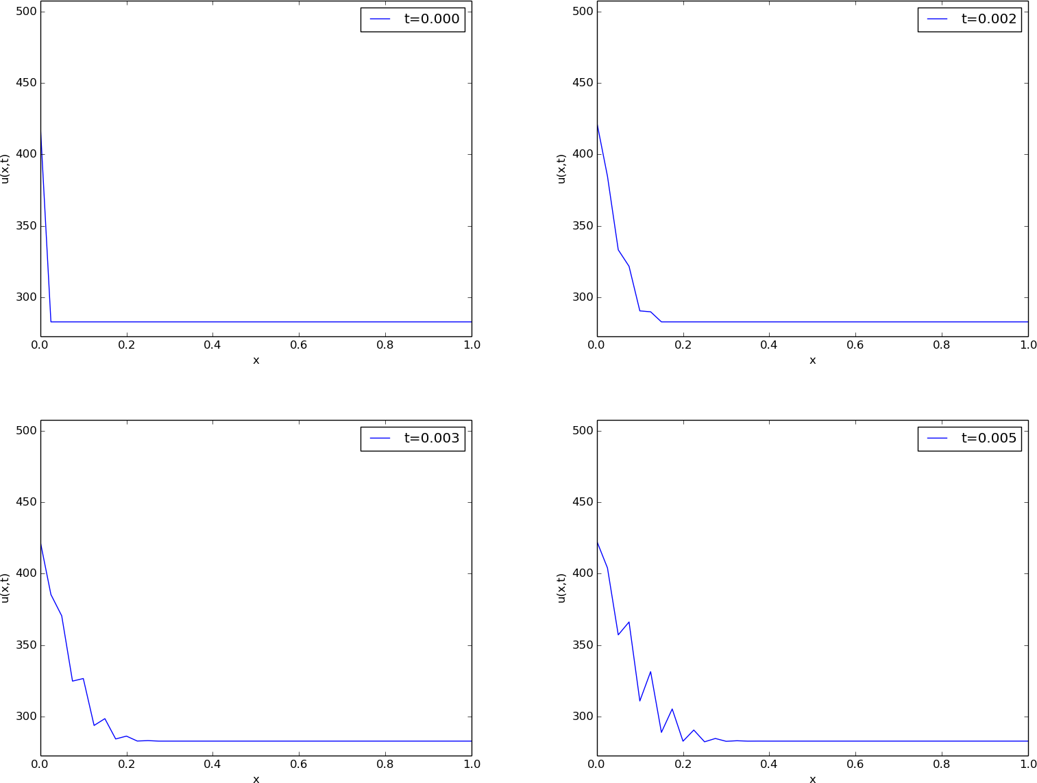
Unstable simulation of the temperature in a rod

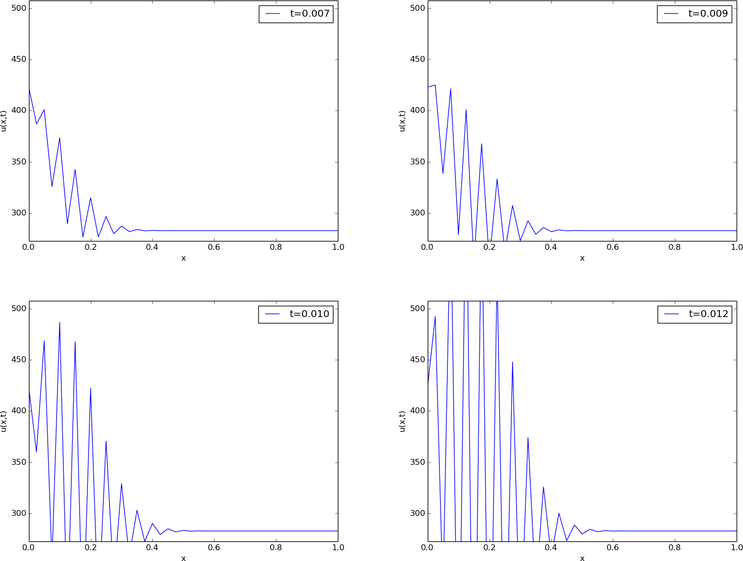
Unstable simulation of the temperature in a rod

The problem is that \(\Delta t\) is too large, making the solution unstable. It turns out that the Forward Euler time integration method puts a restriction on the size of \(\Delta t\). For the heat equation and the way we have discretized it, this restriction can be shown to be [Ref20]

\[\tag{134} \Delta t \leq \frac{\Delta x^2}{2\beta}\thinspace .\]

This is called a stability criterion. With the chosen parameters, (134) tells us that the upper limit is \(\Delta t=0.0003125\), which is smaller than our choice above. Rerunning the case with a \(\Delta t\) equal to \(\Delta x^2/(2\beta)\), indeed shows a smooth evolution of \(u(x,t)\). Find the program rod_FE.py and run it to see an animation of the \(u(x,t)\) function on the screen.

Scaling and dimensionless quantities

Our setting of parameters required finding three physical properties of a certain material. The time interval for simulation and the time step depend crucially on the values for \(\beta\) and \(L\), which can vary significantly from case to case. Often, we are more interested in how the shape of \(u(x,t)\) develops, than in the actual \(u\), \(x\), and \(t\) values for a specific material. We can then simplify the setting of physical parameters by scaling the problem.

Scaling means that we introduce dimensionless independent and dependent variables, here denoted by a bar:

\[\bar u = \frac{u-u^*}{u_c-u^*},\quad \bar x=\frac{x}{x_c},\quad \bar t = \frac{t}{t_c},\]

where \(u_c\) is a characteristic size of the temperature, \(u^*\) is some reference temperature, while \(x_c\) and \(t_c\) are characteristic time and space scales. Here, it is natural to choose \(u^*\) as the initial condition, and set \(u_c\) to the stationary (end) temperature. Then \(\bar u\in [0,1]\), starting at 0 and ending at 1 as \(t\rightarrow\infty\). The length \(L\) is \(x_c\), while choosing \(t_c\) is more challenging, but one can argue for \(t_c = L^2/\beta\). The resulting equation for \(\bar u\) reads

\[\frac{\partial \bar u}{\partial \bar t} = \frac{\partial^2 \bar u}{\partial \bar x^2},\quad \bar x\in (0,1)\thinspace .\]

Note that in this equation, there are no physical parameters! In other words, we have found a model that is independent of the length of the rod and the material it is made of (!).

We can easily solve this equation with our program by setting \(\beta=1\), \(L=1\), \(I(x)=0\), and \(s(t)=1\). It turns out that the total simulation time (to “infinity”) can be taken as 1.2. When we have the solution \(\bar u(\bar x,\bar t)\), the solution with dimension Kelvin, reflecting the true temperature in our medium, is given by

\[u(x,t) = u^* + (u_c-u^*)\bar u(x/L, t\beta/L^2)\thinspace .\]

Through this formula we can quickly generate the solutions for a rod made of aluminum, wood, or rubber - it is just a matter of plugging in the right \(\beta\) value.

Figure Snapshots of the dimensionless solution of a scaled problem shows four snapshots of the scaled (dimensionless) solution \(\bar (\bar x,\bar t)\).

The power of scaling is to reduce the number of physical parameters in a problem, and in the present case, we found one single problem that is independent of the material (\(\beta\)) and the geometry (\(L\)).

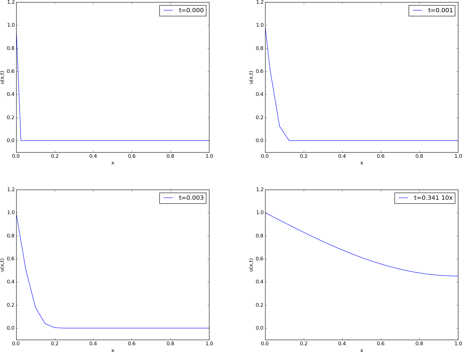
Snapshots of the dimensionless solution of a scaled problem

Vectorization

Occasionally in this book, we show how to speed up code by replacing loops over arrays by vectorized expressions. The present problem involves a loop for computing the right-hand side:

for i in range(1, N):
    rhs[i] = (beta/dx**2)*(u[i+1] - 2*u[i] + u[i-1]) + g(x[i], t)

This loop can be replaced by a vectorized expression with the following reasoning. We want to set all the inner points at once: rhs[1:N-1] (this goes from index 1 up to, but not including, N). As the loop index i runs from 1 to N-1, the u[i+1] term will cover all the inner u values displaced one index to the right (compared to 1:N-1), i.e., u[2:N]. Similarly, u[i-1] corresponds to all inner u values displaced one index to the left: u[0:N-2]. Finally, u[i] has the same indices as rhs: u[1:N-1]. The vectorized loop can therefore be written in terms of slices:

rhs[1:N-1] = (beta/dx**2)*(u[2:N+1] - 2*u[1:N] + u[0:N-1]) +
           g(x[1:N], t)

This rewrite speeds up the code by about a factor of 10. A complete code is found in the file rod_FE_vec.py.

Using Odespy to solve the system of ODEs

Let us now show how to apply a general ODE package like Odespy (see the section Software for solving ODEs) to solve our diffusion problem. As long as we have defined a right-hand side function rhs this is very straightforward:

import odespy
solver = odespy.RKFehlberg(rhs)
solver.set_initial_condition(U_0)
T = 1.2
N_t = int(round(T/float(dt)))
time_points = linspace(0, T, N_t+1)
u, t = solver.solve(time_points)

# Check how many time steps are required by adaptive vs
# fixed-step methods
if hasattr(solver, 't_all'):
    print '# time steps:', len(solver.t_all)
else:
    print '# time steps:', len(t)

The very nice thing is that we can now easily experiment with many different integration methods. Trying out some simple ones first, like RK2 and RK4, quickly reveals that the time step limitation of the Forward Euler scheme also applies to these more sophisticated Runge-Kutta methods, but their accuracy is better. However, the Odespy package offers also adaptive methods. We can then specify a much larger time step in time_points, and the solver will figure out the appropriate step. Above we indicated how to use the adaptive Runge-Kutta-Fehlberg 4-5 solver. While the \(\Delta t\) corresponding to the Forward Euler method requires over 8000 steps for a simulation, we started the RKFehlberg method with 100 times this time step and in the end it required just slightly more than 2500 steps, using the default tolerance parameters. Lowering the tolerance did not save any significant amount of computational work. Figure Time steps used by the Runge-Kutta-Fehlberg method: error tolerance \( 10^{-3} \) (left) and \( 10^{-6} \) (right) shows a comparison of the length of all the time steps for two values of the tolerance. We see that the influence of the tolerance is minor in this computational example, so it seems that the blow-up due to instability is what governs the time step size. The nice feature of this adaptive method is that we can just specify when we want the solution to be computed, and the method figures out on its own what time step that has to be used because of stability restrictions.

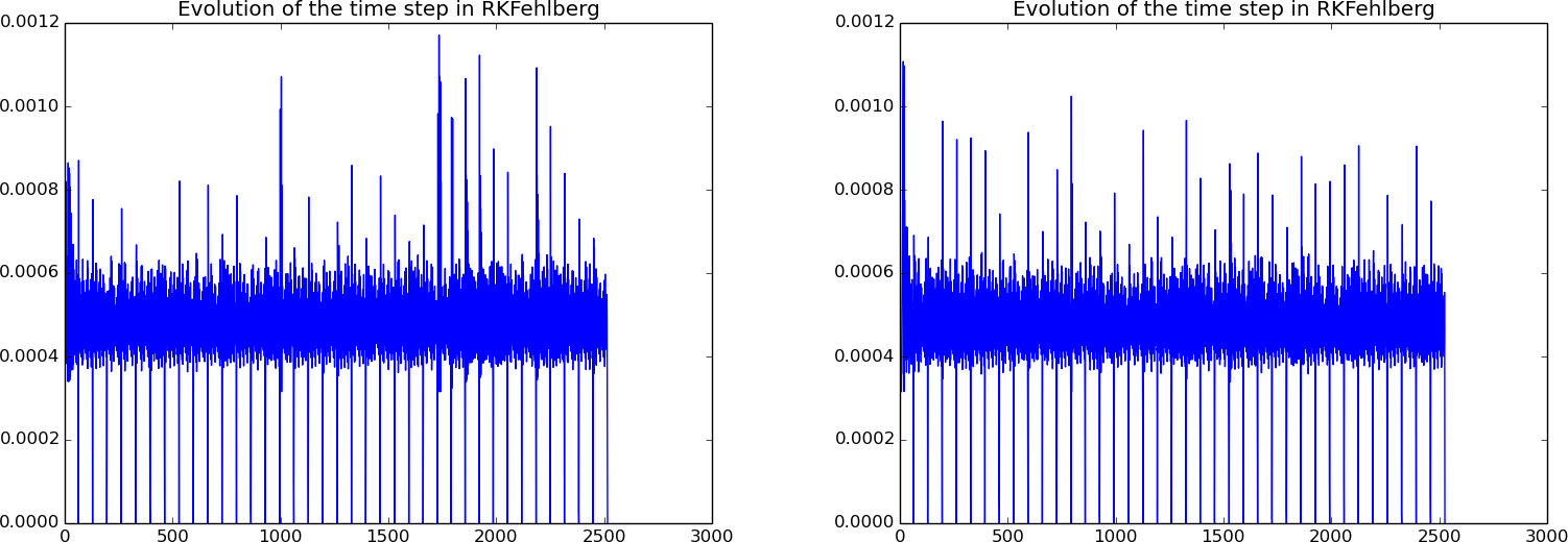
Time steps used by the Runge-Kutta-Fehlberg method: error tolerance \( 10^{-3} \) (left) and \( 10^{-6} \) (right)

We have seen how easy it is to apply sophisticated methods for ODEs to this PDE example. We shall take the use of Odespy one step further in the next section.

Implicit methods

A major problem with the stability criterion (134) is that the time step becomes very small if \(\Delta x\) is small. For example, halving \(\Delta x\) requires four times as many time steps and eight times the work. Now, with \(N=40\), which is a reasonable resolution for the test problem above, the computations are very fast. What takes time, is the visualization on the screen, but for that purpose one can visualize only a subset of the time steps. However, there are occasions when you need to take larger time steps with the diffusion equation, especially if interest is in the long-term behavior as \(t\rightarrow\infty\). You must then turn to implicit methods for ODEs. These methods require the solutions of linear systems, if the underlying PDE is linear, and systems of nonlinear algebraic equations if the underlying PDE is non-linear.

The simplest implicit method is the Backward Euler scheme, which puts no restrictions on \(\Delta t\) for stability, but obviously, a large \(\Delta t\) leads to inaccurate results. The Backward Euler scheme for a scalar ODE \(u' = f(u,t)\) reads

\[\frac{u^{n+1} - u^{n}}{\Delta t} = f(u^{n+1}, t_{n+1})\thinspace .\]

This equation is to be solved for \(u^{n+1}\). If \(f\) is linear in \(u\), it is a linear equation, but if \(f\) is nonlinear in \(u\), one needs approximate methods for nonlinear equations (the chapter Solving nonlinear algebraic equations).

In our case, we have a system of linear ODEs (128)-(130). The Backward Euler scheme applied to each equation leads to

\[\tag{135} \frac{u_0^{n+1}-u_0^n}{\Delta t} = s'(t_{n+1}),\]

\[\tag{136} \frac{u_i^{n+1} - u_i^{n}}{\Delta t} = \frac{\beta}{\Delta x^2} (u_{i+1}^{n+1} - 2u_i^{n+1} + u_{i-1}^{n+1}) + g_i(t_{n+1}),\]

\[\qquad\qquad \quad i=1,\ldots,N-1,\nonumber\]

\[\tag{137} \frac{u_N^{n+1} - u_N^{n}}{\Delta t} = \frac{2\beta}{\Delta x^2} (u_{N-1}^{n+1} - u_N^{n+1}) + g_i(t_{n+1})\thinspace .\]

This is a system of linear equations in the unknowns \(u_i^{n+1}\), \(i=0,\ldots,N\), which is easy to realize by writing out the equations for the case \(N=3\), collecting all the unknown terms on the left-hand side and all the known terms on the right-hand side:

\[\tag{138} u_0^{n+1} = u_0^n + \Delta t\,s'(t_{n+1}),\]

\[\tag{139} u_1^{n+1} - \Delta t \frac{\beta}{\Delta x^2} (u_{2}^{n+1} - 2u_1^{n+1} + u_{0}^{n+1}) = u_1^{n} + \Delta t\,g_1(t_{n+1}),\]

\[\tag{140} u_2^{n+1} - \Delta t\frac{2\beta}{\Delta x^2} (u_{1}^{n+1} - u_2^{n+1}) = u_2^{n} + \Delta t\,g_2(t_{n+1})\thinspace .\]

A system of linear equations like this, is usually written on matrix form \(Au=b\), where \(A\) is a coefficient matrix, \(u=(u_0^{n+1},\ldots,n_N^{n+1})\) is the vector of unknowns, and \(b\) is a vector of known values. The coefficient matrix for the case (138)-(140) becomes

\[\begin{split}A = \left(\begin{array}{ccc} 1 & 0 & 0\\ -\Delta t \frac{\beta}{\Delta x^2} & 1 + 2\Delta t \frac{\beta}{\Delta x^2} & - \Delta t \frac{\beta}{\Delta x^2}\\ 0 & - \Delta t\frac{2\beta}{\Delta x^2} & 1 + \Delta t\frac{2\beta}{\Delta x^2} \end{array}\right)\end{split}\]

In the general case (135)-(137), the coefficient matrix is an \((N+1)\times(N+1)\) matrix with zero entries, except for

\[\tag{141} A_{1,1} = 1\]

\[\tag{142} A_{i,i-1} = -\Delta t \frac{\beta}{\Delta x^2},\quad i=2,\ldots,N-1\]

\[\tag{143} A_{i,i+1} = -\Delta t \frac{\beta}{\Delta x^2},\quad i=2,\ldots,N-1\]

\[\tag{144} A_{i,i} = 1 + 2\Delta t \frac{\beta}{\Delta x^2},\quad i=2,\ldots,N-1\]

\[\tag{145} A_{N,N-1} = - \Delta t\frac{2\beta}{\Delta x^2}\]

\[\tag{146} A_{N,N} = 1 + \Delta t\frac{2\beta}{\Delta x^2}\]

If we want to apply general methods for systems of ODEs on the form \(u'=f(u,t)\), we can assume a linear \(f(u,t)=Ku\). The coefficient matrix \(K\) is found from the right-hand side of (135)-(137) to be

\[\tag{147} K_{1,1} = 0\]

\[\tag{148} K_{i,i-1} = \frac{\beta}{\Delta x^2},\quad i=2,\ldots,N-1\]

\[\tag{149} K_{i,i+1} = \frac{\beta}{\Delta x^2},\quad i=2,\ldots,N-1\]

\[\tag{150} K_{i,i} = -\frac{2\beta}{\Delta x^2},\quad i=2,\ldots,N-1\]

\[\tag{151} K_{N,N-1} = \frac{2\beta}{\Delta x^2}\]

\[\tag{152} K_{N,N} = -\frac{2\beta}{\Delta x^2}\]

We see that \(A=I-\Delta t\,K\).

To implement the Backward Euler scheme, we can either fill a matrix and call a linear solver, or we can apply Odespy. We follow the latter strategy. Implicit methods in Odespy need the \(K\) matrix above, given as an argument jac (Jacobian of \(f\)) in the call to odespy.BackwardEuler. Here is the Python code for the right-hand side of the ODE system (rhs) and the \(K\) matrix (K) as well as statements for initializing and running the Odespy solver BackwardEuler (in the file rod_BE.py):

def rhs(u, t):
    N = len(u) - 1
    rhs = zeros(N+1)
    rhs[0] = dsdt(t)
    for i in range(1, N):
        rhs[i] = (beta/dx**2)*(u[i+1] - 2*u[i] + u[i-1]) + \
                 g(x[i], t)
    rhs[N] = (beta/dx**2)*(2*u[i-1] + 2*dx*dudx(t) -
                           2*u[i]) + g(x[N], t)
    return rhs

def K(u, t):
    N = len(u) - 1
    K = zeros((N+1,N+1))
    K[0,0] = 0
    for i in range(1, N):
        K[i,i-1] = beta/dx**2
        K[i,i] = -2*beta/dx**2
        K[i,i+1] = beta/dx**2
    K[N,N-1] = (beta/dx**2)*2
    K[N,N] = (beta/dx**2)*(-2)
    return K

import odespy
solver = odespy.BackwardEuler(rhs, f_is_linear=True, jac=K)
solver = odespy.ThetaRule(rhs, f_is_linear=True, jac=K, theta=0.5)
solver.set_initial_condition(U_0)
T = 1*60*60
N_t = int(round(T/float(dt)))
time_points = linspace(0, T, N_t+1)
u, t = solver.solve(time_points)

The file rod_BE.py has all the details and shows a movie of the solution. We can run it with any \(\Delta t\) we want, its size just impacts the accuracy of the first steps.

Odespy solvers apply dense matrices

Looking at the entries of the \(K\) matrix, we realize that there are at maximum three entries different from zero in each row. Therefore, most of the entries are zeroes. The Odespy solvers expect dense square matrices as input, here with \((N+1)\times(N+1)\) elements. When solving the linear systems, a lot of storage and work are spent on the zero entries in the matrix. It would be much more efficient to store the matrix as a tridiagonal matrix and apply a specialized Gaussian elimination solver for tridiagonal systems. Actually, this reduces the work from the order \(N^3\) to the order \(N\).

In one-dimensional diffusion problems, the savings of using a tridiagonal matrix are modest in practice, since the matrices are very small anyway. In two- and three-dimensional PDE problems, however, one cannot afford dense square matrices. Rather, one must resort to more efficient storage formats and algorithms tailored to such formats, but this is beyond the scope of the present text.

Exercises

Exercise 63: Simulate a diffusion equation by hand

Consider the problem given by (128), (129) and (133). Set \(N=2\) and compute \(u_i^0\), \(u_i^1\) and \(u_i^2\) by hand for \(i=0,1,2\). Use these values to construct a test function for checking that the implementation is correct. Copy useful functions from test_diffusion_pde_exact_linear.py and make a new test function test_diffusion_hand_calculation.

Solution. Applying the forward Euler method to (128), we get

\[u_0^{n+1}=u_0^n - \Delta t (3L),\quad n=0,1\thinspace .\]

For the requested n values, we then find that

\[u_0^0 = 2(0-L)=-2L=-2(1.5)=-3.0\thinspace ,\nonumber\]

\[u_0^1 = u_0^0 - \Delta t (3L)=-3.0 - 0.1(3(1.5))=-3.45\thinspace ,\nonumber\]

\[u_0^2 = u_0^1 - \Delta t (3L)=-3.45 - 0.1(3(1.5))=-3.90\thinspace .\nonumber\]

Similarly, with forward Euler applied to (129), we get

\[u_1^{n+1}=u_1^n + \frac{\beta \Delta t}{\Delta x^2} (u_2^n - 2u_1^n + u_0^n) + \Delta t (f_1^n),\quad n=0,1\thinspace .\]

For the requested n values, we find

\[u_1^0 = 2(0.75-L)=2(0.75-1.5)=-1.5\thinspace ,\nonumber\]

\[u_1^1 = u_1^0 + \frac{\beta \Delta t}{\Delta x^2} (u_2^0 - 2u_1^0 + u_0^0) + \Delta t (f_1^0)\thinspace ,\nonumber\]

\[= -1.5 + \frac{(0.5)(0.1)}{0.75^2} (0 - 2(-1.5) + (-3.0)) + 0.1 (3(0.75-1.5))\thinspace ,\nonumber\]

\[= -1.725\thinspace ,\nonumber\]

\[u_1^2 = u_1^1 + \frac{\beta \Delta t}{\Delta x^2} (u_2^1 - 2u_1^1 + u_0^1) + \Delta t (f_1^1)\thinspace ,\nonumber\]

\[= -1.725 + \frac{(0.5)(0.1)}{0.75^2} (0 - 2(-1.725) + (-3.45)) + 0.1(3(0.75-1.5))\thinspace ,\nonumber\]

\[= -1.95\thinspace .\nonumber\]

Finally, applying the forward Euler method to (133), we get

\[u_2^{n+1}=u_2^n + \frac{2\beta \Delta t}{\Delta x^2} (u_1^n + \Delta x\gamma - u_2^n) + \Delta t (f_2^n),\quad n=0,1\thinspace .\]

For the requested n values, we find

\[u_2^0 = 2(L-L)=0\thinspace ,\nonumber\]

\[u_2^1 = u_2^0 + \frac{2\beta \Delta t}{\Delta x^2} (u_1^0 + \Delta x\gamma + u_2^0) + \Delta t (f_2^0)\thinspace ,\nonumber\]

\[= 0 + \frac{2(0.5)(0.1)}{0.75^2} (2(0.75-1.5) + \frac{1.5}{2}(3(0) + 2) - 0) + 0.1 (0))\thinspace ,\nonumber\]

\[= 0\thinspace ,\nonumber\]

\[u_2^2 = u_2^1 + \frac{2\beta \Delta t}{\Delta x^2} (u_1^1 + \Delta x\gamma - u_2^1) + \Delta t (f_2^1)\thinspace ,\nonumber\]

\[= 0 + \frac{2(0.5)(0.1)}{0.75^2} (-1.725 + \frac{1.5}{2}(3(0.1)+2)-0) + 0.1(3(1.5-1.5))\thinspace ,\nonumber\]

\[= 0\thinspace .\nonumber\]

Code:

"""Hand calc: Verify implementation of the diffusion equation"""

from ode_system_FE import ode_FE
from numpy import linspace, zeros, abs
#from test_diffusion_pde_exact_linear import rhs, u_exact, dudx, s, dsdt, f

def rhs(u, t):
    N = len(u) - 1
    rhs = zeros(N+1)
    rhs[0] = dsdt(t)
    for i in range(1, N):
        rhs[i] = (beta/dx**2)*(u[i+1] - 2*u[i] + u[i-1]) + \
                 g(x[i], t)
    rhs[N] = (beta/dx**2)*(2*u[N-1] + 2*dx*dudx(t) -
                           2*u[N]) + g(x[N], t)
    return rhs

def u_exact(x, t):
    return (3*t + 2)*(x - L)

def dudx(t):
    return (3*t + 2)

def s(t):
    return u_exact(0, t)

def dsdt(t):
    return 3*(-L)

def g(x, t):
    return 3*(x-L)

def test_rod_diffusion_hand():
    global beta, dx, L, x      # needed in rhs
    L = 1.5
    beta = 0.5
    N = 2
    x = linspace(0, L, N+1)
    dx = x[1] - x[0]
    u = zeros(N+1)

    U_0 = zeros(N+1)
    U_0[0] = s(0)
    U_0[1:] = u_exact(x[1:], 0)

    u_hand = zeros((3, len(U_0)))
    u_hand[0,:] = -3.0, -1.5, 0.0    # spatial indices: 0, 1 and 2
    u_hand[1,:] = -3.45, -1.725, 0.0
    u_hand[2,:] = -3.90, -1.95, 0.0

    dt = 0.1

    u, t = ode_FE(rhs, U_0, dt, T=1.2)

    tol = 1E-12
    for i in [0, 1, 2]:
        print u_hand[i,:]
        print u[i,:]
        diff = abs(u_hand[i,:] - u[i,:]).max()
        assert diff < tol, 'diff=%.16g' % diff
        print 'diff=%g at t=%g' % (diff, t[i])

if __name__ == '__main__':
    test_rod_diffusion_hand()

Filename: test_rod_hand_calculations.py.

Exercise 64: Compute temperature variations in the ground

The surface temperature at the ground shows daily and seasonal oscillations. When the temperature rises at the surface, heat is propagated into the ground, and the coefficient \(\beta\) in the diffusion equation determines how fast this propagation is. It takes some time before the temperature rises down in the ground. At the surface, the temperature has then fallen. We are interested in how the temperature varies down in the ground because of temperature oscillations on the surface.

Assuming homogeneous horizontal properties of the ground, at least locally, and no variations of the temperature at the surface at a fixed point of time, we can neglect the horizontal variations of the temperature. Then a one-dimensional diffusion equation governs the heat propagation along a vertical axis called \(x\). The surface corresponds to \(x=0\) and the \(x\) axis point downwards into the ground. There is no source term in the equation (actually, if rocks in the ground are radioactive, they emit heat and that can be modeled by a source term, but this effect is neglected here).

At some depth \(x=L\) we assume that the heat changes in \(x\) vanish, so \(\partial u/\partial x=0\) is an appropriate boundary condition at \(x=L\). We assume a simple sinusoidal temperature variation at the surface:

\[u(0,t) = T_0 + T_a\sin\left(\frac{2\pi}{P}t\right),\]

where \(P\) is the period, taken here as 24 hours (\(24\cdot 60\cdot 60\) s). The \(\beta\) coefficient may be set to \(10^{-6}\hbox{ m}^2/\hbox{s}\). Time is then measured in seconds. Set appropriate values for \(T_0\) ad \(T_a\).

a) Show that the present problem has an analytical solution of the form

\[u(x,t) = A + Be^{-rx}\sin(\omega t - rx),\]

for appropriate values of \(A\), \(B\), \(r\), and \(\omega\).

Solution. Any function that is supposed to be a solution, must fit the equation, boundary conditions and initial conditions, so we go ahead and check this.

From before, we have the temperature at the surface as a given sine function, i.e. using \(x = 0\) in the suggested (or given) solution should make it equal to the temperature function previously given for the surface. This implies immediately that \(A = T_0\), \(B = T_a\) and \(\omega = \frac{2\pi}{P}\).

At the other boundary, we see that the suggested solution approaches zero when x goes to infinity, which is consistent with the boundary condition \(\frac{\partial u}{\partial x} = 0\).

With \(t = 0\), we find that

\[u(x,0) = A + B e^{-rx}\sin\left(-rx\right),\]

So, by making this our initial temperature distribution, also the initial conditions will be consistent with the suggested solution.

Finally, the suggested solution must be consistent with \(\frac{\partial u}{\partial t} = \beta\frac{\partial^2 u}{\partial x^2}\), so we perform the required partial derivatives to check.

\[\frac{\partial u}{\partial t} = \omega B e^{-rx}\cos\left(\omega t -rx\right),\]

\[\frac{\partial u}{\partial x} = -r B e^{-rx}\sin\left(\omega t -rx\right) -r B e^{-rx}\cos\left(\omega t -rx\right) ,\]

\[\frac{\partial^2 u}{\partial x^2} = -r\left[-r B e^{-rx}\sin\left(\omega t - rx\right) - r B e^{-rx}\cos\left(\omega t - rx\right)\right] - r\left[-r B e^{-rx}\cos\left(\omega t - rx\right) + r B e^{-rx}\sin\left(\omega t -rx\right)\right] ,\]

which reduces to

\[\frac{\partial^2 u}{\partial x^2} = 2 r^2 B e^{-rx}\cos\left(\omega t - rx\right) ,\]

This means that we can decide the final parameter \(r\) as well, since if only \(r = \sqrt{\frac{\omega}{2\beta}}\), we have that \(\frac{\partial u}{\partial t} = \beta\frac{\partial^2 u}{\partial x^2}\).

b) Solve this heat propagation problem numerically for some days and animate the temperature. You may use the Forward Euler method in time. Plot both the numerical and analytical solution. As initial condition for the numerical solution, use the exact solution during program development, and when the curves coincide in the animation for all times, your implementation works, and you can then switch to a constant initial condition: \(u(x,0)=T_0\). For this latter initial condition, how many periods of oscillations are necessary before there is a good (visual) match between the numerical and exact solution (despite differences at \(t=0\))?

Solution. Code:

"""Temperature vertically down in the ground (with Forward Euler)."""

from numpy import linspace, zeros, linspace, exp, sin, cos, pi, sqrt
import time

def U(x, t):
    """ True temperature """
    return A + B*exp(-r*x)*sin(omega*t - r*x)

def rhs(u, t):
    N = len(u) - 1
    rhs = zeros(N+1)
    rhs[0] = dsdt(t)
    for i in range(1, N):
        rhs[i] = (beta/dx**2)*(u[i+1] - 2*u[i] + u[i-1]) + \
                 f(x[i], t)
    i = N
    rhs[i] = (beta/dx**2)*(2*u[i-1] - 2*u[i]) + f(x[N], t)
    return rhs

def dudx(t):
    return 0

def s(t):
    return T0 + Ta*sin((2*pi/P)*t)

def dsdt(t):
    return (Ta*2*pi/P)*cos((2*pi/P)*t)

def f(x, t):
    return 0

def I(x):
    """Initial temp distribution"""
    return A + B*exp(-r*x)*sin(-r*x)

def I(x):
    """Initial temp distribution."""
    return A

beta = 1E-6
T0 = 283        # just some choice
Ta = 20         # amplitude of temp osc
P = 24*60*60    # period, 24 hours
A = T0
B = Ta
omega = 2*pi/P
r = sqrt(omega/(2*beta))
L = 2           # depth vertically down in the ground
N = 100
x = linspace(0, L, N+1)
dx = x[1] - x[0]
u = zeros(N+1)

U_0 = zeros(N+1)
U_0[0] = s(0)
U_0[1:] = I(x[1:])

dt = dx**2/float(2*beta)
print 'stability limit:', dt

t0 = time.clock()
from ode_system_FE import ode_FE
T=(24*60*60)*6                  # simulate 6 days
u, t = ode_FE(rhs, U_0, dt, T)
t1 = time.clock()
print 'CPU time: %.1fs' % (t1 - t0)


# Make movie
import os
os.system('rm tmp_*.png')
import matplotlib.pyplot as plt
plt.ion()
lines = plt.plot(x, u[0,:], x, U(x, 0))
plt.axis([x[0], x[-1], 283-30, 283+30])
plt.xlabel('x')
plt.ylabel('u(x,t) and U(x,t)')
counter = 0
for i in range(0, u.shape[0]):
    print t[i]
    lines[0].set_ydata(u[i,:])
    lines[1].set_ydata(U(x, t[i]))
    plt.legend(['t=%.3f' % t[i]])
    plt.draw()
    if i % 10 == 0: # plot every x steps
        #plt.savefig('tmp_%04d.png' % counter)
        counter += 1
    #time.sleep(0.2)

Filename: ground_temp.py.

Exercise 65: Compare implicit methods

An equally stable, but more accurate method than the Backward Euler scheme, is the so-called 2-step backward scheme, which for an ODE \(u'=f(u,t)\) can be expressed by

\[\frac{3u^{n+1} - 4u^{n} + u^{n-1}}{2\Delta t} = f(u^{n+1},t_{n+1}) \thinspace .\]

The Odespy package offers this method as odespy.Backward2Step. The purpose of this exercise is to compare three methods and animate the three solutions:

1. The Backward Euler method with \(\Delta t =0.001\)
2. The backward 2-step method with \(\Delta t =0.001\)
3. The backward 2-step method with \(\Delta t =0.01\)

Choose the model problem from the section Application: heat conduction in a rod.

Solution. Here is the code:

"""
Temperature evolution in a rod,
computed by a BackwardEuler method and a 2-step
backward method.
"""

from numpy import linspace, zeros, linspace

def rhs(u, t):
    N = len(u) - 1
    rhs = zeros(N+1)
    rhs[0] = dsdt(t)
    for i in range(1, N):
        rhs[i] = (beta/dx**2)*(u[i+1] - 2*u[i] + u[i-1]) + \
                 f(x[i], t)
    rhs[N] = (beta/dx**2)*(2*u[N-1] + 2*dx*dudx(t) -
                           2*u[N]) + g(x[N], t)
    return rhs

def K(u, t):
    N = len(u) - 1
    K = zeros((N+1,N+1))
    K[0,0] = 0
    for i in range(1, N):
        K[i,i-1] = beta/dx**2
        K[i,i] = -2*beta/dx**2
        K[i,i+1] = beta/dx**2
    K[N,N-1] = (beta/dx**2)*2
    K[N,N] = (beta/dx**2)*(-2)
    return K

def dudx(t):
    return 0

def s(t):
    return 323

def dsdt(t):
    return 0

def g(x, t):
    return 0


L = 0.5
beta = 8.2E-5
N = 40
x = linspace(0, L, N+1)
dx = x[1] - x[0]
u = zeros(N+1)

U_0 = zeros(N+1)
U_0[0] = s(0)
U_0[1:] = 283
dt = dx**2/(2*beta)
print 'stability limit:', dt
dt = 12

import odespy
solver0 = odespy.BackwardEuler(rhs, f_is_linear=True, jac=K)
solver1 = odespy.Backward2Step(rhs, f_is_linear=True, jac=K)
solver2 = odespy.Backward2Step(rhs, f_is_linear=True, jac=K)
solver0.set_initial_condition(U_0)
solver1.set_initial_condition(U_0)
solver2.set_initial_condition(U_0)
T = 1*60*60
N_t = int(round(T/float(dt)))
time_points = linspace(0, T, N_t+1)
u0, t0 = solver0.solve(time_points)
u1, t1 = solver1.solve(time_points)
# Solve with larger time step in the 2-step method
factor = 10
dt = factor*dt
N_t = int(round(T/float(dt)))
time_points = linspace(0, T, N_t+1)
u2, t2 = solver2.solve(time_points)

# Make movie
import os
os.system('rm tmp_*.png')
import matplotlib.pyplot as plt
import time
plt.ion()
lines = plt.plot(x, u0[0,:], x, u1[0,:], x, u2[0,:])
plt.axis([x[0], x[-1], 273, s(0)+10])
plt.xlabel('x')
plt.ylabel('u(x,t)')
counter = 0
for i in range(len(t2)):
    print t2[i]
    lines[2].set_ydata(u2[i,:])
    lines[0].set_ydata(u0[factor*i,:])
    lines[1].set_ydata(u1[factor*i,:])
    plt.title('t=%.3f' % t2[i])
    plt.legend(['BE', 'B2Step', 'B2Step 2*dt'])
    plt.draw()
    time.sleep(0.5)
    plt.savefig('tmp_%04d.png' % counter)
    counter += 1

Filename: rod_BE_vs_B2Step.py.

Exercise 66: Explore adaptive and implicit methods

We consider the same problem as in Exercise 64: Compute temperature variations in the ground. Now we want to explore the use of adaptive and implicit methods from Odespy to see if they are more efficient than the Forward Euler method. Assume that you want the accuracy provided by the Forward Euler method with its maximum \(\Delta t\) value. Since there exists an analytical solution, you can compute an error measure that summarizes the error in space and time over the whole simulation:

\[E = \sqrt{\Delta x\Delta t\sum_{i}\sum_n (U_i^n - u_i^n)^2}\thinspace .\]

Here, \(U_i^n\) is the exact solution. Use the Odespy package to run the following implicit and adaptive solvers:

1. BackwardEuler
2. Backward2Step
3. RKFehlberg

Experiment to see if you can use larger time steps than what is required by the Forward Euler method and get solutions with the same order of accuracy.

Hint. To avoid oscillations in the solutions when using the RKFehlberg method, the rtol and atol parameters to RKFFehlberg must be set no larger than 0.001 and 0.0001, respectively. You can print out solver_RKF.t_all to see all the time steps used by the RKFehlberg solver (if solver is the RKFehlberg object). You can then compare the number of time steps with what is required by the other methods.

Solution. Code:

"""
Temperature vertically down in the ground with Forward Euler,
Backward Euler, backward 2-step and RKFehlberg .
"""

from numpy import linspace, zeros, linspace, sin, cos, pi, \
                  exp, sqrt
import time

def rhs(u, t):
    N = len(u) - 1
    rhs = zeros(N+1)
    rhs[0] = dsdt(t)
    for i in range(1, N):
        rhs[i] = (beta/dx**2)*(u[i+1] - 2*u[i] + u[i-1]) + \
                 g(x[i], t)
    i = N
    rhs[i] = (beta/dx**2)*(2*u[i-1] - 2*u[i]) + g(x[N], t)
    return rhs

def K(u, t):
    N = len(u) - 1
    K = zeros((N+1, N+1))
    K[0, 0] = 0
    for i in range(1, N):
        K[i, i-1] = beta/dx**2
        K[i, i]   = -2*beta/dx**2
        K[i, i+1] = beta/dx**2
    K[N, N-1] = (beta/dx**2)*2
    K[N, N]   = (beta/dx**2)*(-2)
    return K

def dudx(t):
    return 0

def s(t):
    return T0 + Ta*sin((2*pi/P)*t)

def dsdt(t):
    return (Ta*2*pi/P)*cos((2*pi/P)*t)

def g(x, t):
    return 0

def U(x, t):
    """ True temperature."""
    return A + B*exp(-r*x)*sin(omega*t - r*x)

def I(x):
    """Initial temp distribution."""
    return U(x, 0)

T0 = 283        # just some choice
Ta = 20         # amplitude of temp osc
P = 24*60*60    # period, 24 hours
A = T0
B = Ta
omega = 2*pi/P
beta = 1E-6
r = sqrt(omega/(2*beta))
L = 2           # depth vertically down in the ground
N = 100
x = linspace(0, L, N+1)
dx = x[1] - x[0]
u = zeros(N+1)

U_0 = zeros(N+1)
U_0[0] = s(0)
U_0[1:] = I(x[1:])
FE_stability_limit = dx**2/float(2*beta)
dt = 1*FE_stability_limit
print 'dt/(FE stability limit): %.1f' % (dt/FE_stability_limit)
T=(24*60*60)*6   # simulate 6 days

import odespy
solver1 = odespy.BackwardEuler(rhs, f_is_linear=True, jac=K)
solver2 = odespy.Backward2Step(rhs, f_is_linear=True, jac=K)
solver3 = odespy.RKFehlberg(rhs, rtol=0.001, atol=0.0001)
solver1.set_initial_condition(U_0)
solver2.set_initial_condition(U_0)
solver3.set_initial_condition(U_0)
N_t = int(round(T/float(dt)))
time_points = linspace(0, T, N_t+1)
u1, t1 = solver1.solve(time_points)
u2, t2 = solver2.solve(time_points)
u3, t3 = solver3.solve(time_points)
print 'N_t=%d, RKF N_t:%d' % (N_t, len(solver3.t_all))
print 'Average dt for RKF: %.2f' % (T/float(len(solver3.t_all)))

if dt <= FE_stability_limit:
    from ode_system_FE import ode_FE
    u4, t4 = ode_FE(rhs, U_0, dt, T)

# Compute error with each method
E1 = 0; E2 = 0; E3 = 0; E_FE = 0
for i in range(len(x)):
    for n in range(len(time_points)):
        if dt <= FE_stability_limit:
            E_FE += (U(x[i], time_points[n]) - u4[n,i])**2
        E1 += (U(x[i], time_points[n]) - u1[n,i])**2
        E2 += (U(x[i], time_points[n]) - u2[n,i])**2
        E3 += (U(x[i], time_points[n]) - u3[n,i])**2
if dt <= FE_stability_limit:
    E_FE = sqrt(dx*dt*E_FE)
E1 = sqrt(dx*dt*E1)
E2 = sqrt(dx*dt*E2)
E3 = sqrt(dx*dt*E3)

#print E0  # gives 31.86 with dt on stability limit
if dt <= FE_stability_limit:
    ref_error = E_FE
else:
    ref_error = 66.31
print  'ref_error:', ref_error

if E1 > (ref_error*10):
    print 'ref_error: %.2f , dt = %.4f at stability lim' % \
                          (ref_error, FE_stability_limit)
    print 'E1 (with BE) too large: %.2f, dt = %.4f' % (E1, dt)
elif E2 > (ref_error*10):
    print 'ref_error: %.2f , dt = %.4f at stability lim' % \
                          (ref_error, FE_stability_limit)
    print 'E2 (with B2Step) too large: %.2f, dt = %.4f' % (E2, dt)
elif E3 > (ref_error*10):
    print 'ref_error: %.2f , dt = %.4f at stability lim' % \
                          (ref_error, FE_stability_limit)
    print 'E3 (with RKF) too large: %.2f, dt = %.4f' % (E3, dt)

# Make movie
import os
os.system('rm tmp_*.png')
import matplotlib.pyplot as plt
plt.ion()
u0 = U(x, 0)
if dt <= FE_stability_limit:
    lines = plt.plot(x, u0, x, u1[0,:], x, u2[0,:], x, u3[0,:], x, u4[0,:])
else:
    lines = plt.plot(x, u0, x, u1[0,:], x, u2[0,:], x, u3[0,:])
plt.axis([x[0], x[-1], 283-30, 283+30])
plt.xlabel('x')
plt.ylabel('u(x,t)')
counter = 0
for i in range(len(t1)):
    u0 = U(x, t1[i])
    lines[0].set_ydata(u0)
    lines[1].set_ydata(u1[i,:])
    lines[2].set_ydata(u2[i,:])
    lines[3].set_ydata(u3[i,:])
    if dt <= FE_stability_limit:
        lines[4].set_ydata(u4[i,:])
    plt.title('t=%.1f days' % (t1[i]/(60*60*24.)))
    if dt <= FE_stability_limit:
        plt.legend(['exact', 'BE', 'B2Step', 'RKF', 'FE'])
    else:
        plt.legend(['exact', 'BE', 'B2Step', 'RKF'])
    plt.draw()
    #time.sleep(0.1)
    plt.savefig('tmp_%04d.png' % counter)
    counter += 1

From experiments it is clear that RKFehlberg uses many more steps, even at the Forward Euler stability limit than the other schemes without giving more accuracy. It seems that the 2-step Backward method is the best one.

Filename: ground_temp_adaptive.py.

Exercise 67: Investigate the \(\theta\) rule

a) The Crank-Nicolson method for ODEs is very popular when combined with diffusion equations. For a linear ODE \(u'=au\) it reads

\[\frac{u^{n+1}-u^n}{\Delta t} = \frac{1}{2}(au^{n} + au^{n+1}) \thinspace .\]

Apply the Crank-Nicolson method in time to the ODE system for a one-dimensional diffusion equation. Identify the linear system to be solved.

Solution. Our system of ODEs reads

\[\frac{du_0}{dt} = s'(t), \nonumber\]

\[\frac{du_i}{dt} = \frac{\beta}{\Delta x^2} (u_{i+1}(t) - 2u_i(t) + u_{i-1}(t)) + f_i(t),\quad i=1,\ldots,N-1, \nonumber\]

\[\frac{du_N}{dt} = \frac{2\beta}{\Delta x^2} (u_{N-1}(t) - u_N(t)) + f_N(t)\thinspace . \nonumber\]

To ease reading, we now proceed by writing the variables without showing explicitly the dependence on time \(t\). With the Crank-Nicolson method, we get

\[\frac{u_0^{n+1} - u_0^n}{\Delta t} = \frac{1}{2}\left(s^n + s^{n+1}\right), \nonumber\]

\[\frac{u_i^{n+1} - u_i^n}{\Delta t} = \frac{1}{2} \biggl(\frac{\beta}{\Delta x^2} (u_{i+1}^n - 2u_i^n + u_{i-1}^n) + f_i^n +\nonumber\]

\[\quad \frac{\beta}{\Delta x^2} (u_{i+1}^{n+1} - 2u_i^{n+1} + u_{i-1}^{n+1}) + f_i^{n+1}\biggr),\quad i=1,\ldots,N-1, \nonumber\]

\[\frac{u_N^{n+1} - u_N^n}{\Delta t} = \frac{1}{2} \left(\frac{2\beta}{\Delta x^2}(u_{N-1}^n - u_N^n) + f_N^n + \frac{2\beta}{\Delta x^2}(u_{N-1}^{n+1} - u_N^{n+1}) + f_N^{n+1}\right)\thinspace . \nonumber\]

Collecting the unknowns on the left hand side, brings us to

\[u_0^{n+1} = u_0^n + \frac{\Delta t}{2}\left(s^n + s^{n+1}\right), \nonumber\]

\[-\frac{\Delta t\beta}{2\Delta x^2}u_{i-1}^{n+1} + (1+\frac{\Delta t\beta}{\Delta x^2})u_i^{n+1} - \frac{\Delta t\beta}{2\Delta x^2}u_{i+1}^{n+1} = u_i^n + \frac{\Delta t\beta}{2\Delta x^2}(u_{i+1}^n - 2u_i^n + u_{i-1}^n) +\nonumber\]

\[\quad \frac{\Delta t}{2}(f_i^n + f_i^{n+1}),\quad i=1,\ldots,N-1, \nonumber\]

\[-\frac{\Delta t\beta}{\Delta x^2}u_{N-1}^{n+1} + (1+\frac{\Delta t\beta}{\Delta x^2})u_N^{n+1} = u_N^n + \frac{\Delta t\beta}{\Delta x^2}(u_{N-1}^n - u_N^n) +\nonumber\]

\[\quad \frac{\Delta t}{2}(f_N^n + f_N^{n+1})\thinspace . \nonumber\]

This is a system of linear equations \(Au = b\), where \(A\) is filled with zeros, except for the elements

\[A_{1,1} = 1\nonumber\]

\[A_{i,i-1} = -\Delta t \frac{\beta}{\Delta x^2},\quad i=2,\ldots,N-1\nonumber\]

\[A_{i,i+1} = -\Delta t \frac{\beta}{\Delta x^2},\quad i=2,\ldots,N-1\nonumber\]

\[A_{i,i} = 1 + \Delta t \frac{\beta}{\Delta x^2},\quad i=2,\ldots,N-1\nonumber\]

\[A_{N,N-1} = - \Delta t\frac{\beta}{\Delta x^2}\nonumber\]

\[A_{N,N} = 1 + \Delta t\frac{\beta}{\Delta x^2}\nonumber\]

and

\[b_1 = u_0^n + \frac{\Delta t}{2}\left(s^n + s^{n+1}\right)\nonumber\]

\[b_i = u_i^n +\Delta t \frac{\beta}{2\Delta x^2}\left(u_{i+1}^n - 2u_i^n + u_{i-1}^n\right) + \frac{\Delta t}{2}\left(f_i^n + f_i^{n+1}\right) ,\quad i=2,\ldots,N-1\nonumber\]

\[b_N = u_N^n + \Delta t\frac{\beta}{\Delta x^2}\left(u_{N-1}^n - u_N^n\right) + \frac{\Delta t}{2}\left(f_N^n + f_N^{n+1}\right)\nonumber\]

b) The Backward Euler, Forward Euler, and Crank-Nicolson methods can be given a unified implementation. For a linear ODE \(u'=au\) this formulation is known as the \(\theta\) rule:

\[\frac{u^{n+1}-u^n}{\Delta t} = (1-\theta)au^{n} + \theta au^{n+1} \thinspace .\]

For \(\theta =0\) we recover the Forward Euler method, \(\theta=1\) gives the Backward Euler scheme, and \(\theta=1/2\) corresponds to the Crank-Nicolson method. The approximation error in the \(\theta\) rule is proportional to \(\Delta t\), except for \(\theta =1/2\) where it is proportional to \(\Delta t^2\). For \(\theta \geq 1/2\) the method is stable for all \(\Delta t\).

Apply the \(\theta\) rule to the ODE system for a one-dimensional diffusion equation. Identify the linear system to be solved.

Solution. With the theta rule, we get

\[\frac{u_0^{n+1} - u_0^n}{\Delta t} = (1-\theta) s^n + \theta s^{n+1}, \nonumber\]

\[\frac{u_i^{n+1} - u_i^n}{\Delta t} = (1-\theta)\left(\frac{\beta}{\Delta x^2} (u_{i+1}^n - 2u_i^n + u_{i-1}^n) + f_i^n\right) +\nonumber\]

\[\quad \theta \left(\frac{\beta}{\Delta x^2} (u_{i+1}^{n+1} - 2u_i^{n+1} + u_{i-1}^{n+1}) + f_i^{n+1}\right),\quad i=1,\ldots,N-1, \nonumber\]

\[\frac{u_N^{n+1} - u_N^n}{\Delta t} = (1-\theta)\left(\frac{2\beta}{\Delta x^2}(u_{N-1}^n - u_N^n) + f_N^n\right) + \theta \left(\frac{2\beta}{\Delta x^2}(u_{N-1}^{n+1} - u_N^{n+1}) + f_N^{n+1}\right)\thinspace . \nonumber\]

Collecting the unknowns on the left hand side gives

\[u_0^{n+1} = u_0^n + \Delta t\left((1-\theta) s^n + \theta s^{n+1}\right),\nonumber\]

\[-\theta\frac{\Delta t\beta}{\Delta x^2}u_{i-1}^{n+1} + \left(1+\theta\frac{2\Delta t\beta}{\Delta x^2}u_i^{n+1}\right) - \theta\frac{\Delta t\beta}{\Delta x^2}u_{i+1}{n+1} = u_i^n +\nonumber\]

\[\Delta t\left(1-\theta\right)\frac{\beta}{\Delta x^2}\left(u_{i+1}^n - 2u_i^n + u_{i-1}^n\right) + \Delta t\left((1-\theta)f_i^n + \theta f_i^{n+1}\right),\quad i=1,\ldots,N-1,\nonumber\]

\[-\theta\frac{2\Delta t\beta}{\Delta x^2}u_{N-1}^{n+1} + \left(1+\theta\frac{2\Delta t\beta}{\Delta x^2}u_N^{n+1}\right) = u_N^n +\nonumber\]

\[\Delta t(1-\theta)\frac{2\beta}{\Delta x^2}\left(u_{N-1}^n - u_N^n\right) + \Delta t\left((1-\theta)f_N^n + \theta f_N^{n+1}\right)\thinspace , \nonumber\]

which is a system of linear equations \(Au = b\), where \(A\) is filled with zeros, except for the elements

\[A_{1,1} = 1\nonumber\]

\[A_{i,i-1} = -\theta \Delta t \frac{\beta}{\Delta x^2},\quad i=2,\ldots,N-1\nonumber\]

\[A_{i,i+1} = -\theta \Delta t \frac{\beta}{\Delta x^2},\quad i=2,\ldots,N-1\nonumber\]

\[A_{i,i} = 1 + \theta \Delta t \frac{2\beta}{\Delta x^2},\quad i=2,\ldots,N-1\nonumber\]

\[A_{N,N-1} = - \theta \Delta t\frac{2\beta}{\Delta x^2}\nonumber\]

\[A_{N,N} = 1 + \theta \Delta t\frac{2\beta}{\Delta x^2}\nonumber\]

and

\[b_1 = u_0^n + \Delta t\left((1-\theta)s^n + \theta s^{n+1}\right)\nonumber\]

\[b_i = u_i^n +\Delta t(1-\theta) \frac{\beta}{\Delta x^2}\left(u_{i+1}^n - 2u_i^n + u_{i-1}^n\right) + \Delta t\left((1-\theta)f_i^n + \theta f_i^{n+1}\right),\quad i=2,\ldots,N-1\nonumber\]

\[b_N = u_N^n + \Delta t(1-\theta)\frac{2\beta}{\Delta x^2}\left(u_{N-1}^n - u_N^n\right) + \Delta t\left((1-\theta)f_N^n + \theta f_N^{n+1}\right)\nonumber\]

c) Implement the \(\theta\) rule with aid of the Odespy package. The relevant object name is ThetaRule:

solver = odespy.ThetaRule(rhs, f_is_linear=True, jac=K, theta=0.5)

d) Consider the physical application from the section Application: heat conduction in a rod. Run this case with the \(\theta\) rule and \(\theta =1/2\) for the following values of \(\Delta t\): 0.001, 0.01, 0.05. Report what you see.

Solution. With the two larger time steps we see some non-physical oscillations near the end with constant temperature. These oscillations die out as the stationary case is approached. With a time step of \(0.001\), there are no oscillations at all.

Code:

"""Temperature evolution in a rod, computed by a BackwardEuler method."""

from numpy import linspace, zeros, linspace

def rhs(u, t):
    N = len(u) - 1
    rhs = zeros(N+1)
    rhs[0] = dsdt(t)
    for i in range(1, N):
        rhs[i] = (beta/dx**2)*(u[i+1] - 2*u[i] + u[i-1]) + \
                 f(x[i], t)
    rhs[N] = (beta/dx**2)*(2*u[i-1] + 2*dx*dudx(t) -
                           2*u[i]) + f(x[N], t)
    return rhs

def K(u, t):
    N = len(u) - 1
    K = zeros((N+1,N+1))
    K[0,0] = 0
    for i in range(1, N):
        K[i,i-1] = beta/dx**2
        K[i,i] = -2*beta/dx**2
        K[i,i+1] = beta/dx**2
    K[N,N-1] = (beta/dx**2)*2
    K[N,N] = (beta/dx**2)*(-2)
    return K

def K_vec(u, t):
    """Vectorized computation of K."""
    N = len(u) - 1
    K = zeros((N+1,N+1))
    K[0,0] = 0
    K[1:N-1] = beta/dx**2
    K[1:N] = -2*beta/dx**2
    K[2:N+1] = beta/dx**2
    K[N,N-1] = (beta/dx**2)*2
    K[N,N] = (beta/dx**2)*(-2)
    return K

def dudx(t):
    return 0

def s(t):
    return 423

def dsdt(t):
    return 0

def f(x, t):
    return 0


L = 1
beta = 1
N = 40
x = linspace(0, L, N+1)
dx = x[1] - x[0]
u = zeros(N+1)

U_0 = zeros(N+1)
U_0[0] = s(0)
U_0[1:] = 283
dt = dx**2/(2*beta)
print 'stability limit:', dt
dt = 0.05
#dt = 0.00034375  # ForwardEuler limit

import odespy
solver = odespy.ThetaRule(rhs, f_is_linear=True, jac=K, theta=0.5)
solver.set_initial_condition(U_0)
T = 1.2
N_t = int(round(T/float(dt)))
time_points = linspace(0, T, N_t+1)
u, t = solver.solve(time_points)

# Make movie
import os
os.system('rm tmp_*.png')
import matplotlib.pyplot as plt
import time
plt.ion()
y = u[0,:]
lines = plt.plot(x, y)
plt.axis([x[0], x[-1], 273, 1.2*s(0)])
plt.xlabel('x')
plt.ylabel('u(x,t)')
counter = 0
for i in range(0, u.shape[0]):
    print t[i]
    lines[0].set_ydata(u[i,:])
    plt.legend(['t=%.3f' % t[i]])
    plt.draw()
    plt.savefig('tmp_%04d.png' % counter)
    counter += 1
    time.sleep(0.2)

Filename: rod_ThetaRule.py.

Remarks

Despite the fact that the Crank-Nicolson method, or the \(\theta\) rule with \(\theta=1/2\), is theoretically more accurate than the Backward Euler and Forward Euler schemes, it may exhibit non-physical oscillations as in the present example if the solution is very steep. The oscillations are damped in time, and decreases with decreasing \(\Delta t\). To avoid oscillations one must have \(\Delta t\) at maximum twice the stability limit of the Forward Euler method. This is one reason why the Backward Euler method (or a 2-step backward scheme, see Exercise 65: Compare implicit methods) are popular for diffusion equations with abrupt initial conditions.

Exercise 68: Compute the diffusion of a Gaussian peak

Solve the following diffusion problem:

\[\tag{153} \frac{\partial u}{\partial t} = \beta\frac{\partial^2 u}{\partial x^2}, x\in (-1,1),\ t\in (0,T]\]

\[\tag{154} u(x,0) = \frac{1}{\sqrt{2\pi}\sigma}\exp{\left(-\frac{x^2}{2\sigma^2}\right)}, x\in [-1,1],\]

\[\tag{155} \frac{\partial}{\partial x}u(-1,t) = 0 t\in (0,T],\]

\[\tag{156} \frac{\partial}{\partial x}u(1,t) = 0 t\in (0,T]\thinspace .\]

The initial condition is the famous and widely used Gaussian function with standard deviation (or “width”) \(\sigma\), which is here taken to be small, \(\sigma = 0.01\), such that the initial condition is a peak. This peak will then diffuse and become lower and wider. Compute \(u(x,t)\) until \(u\) becomes approximately constant over the domain.

Solution. Code:

"""
Initially, u has a Gaussian distribution and we
follow the distribution over x = [-1,1] until u
is approximately zero.
"""

from numpy import linspace, zeros, linspace, exp, sqrt, pi

def rhs(u, t):
    N = len(u) - 1
    rhs = zeros(N+1)
    rhs[0] = (2*beta/dx**2)*(u[1] - u[0]) + g(x[0], t)
    for i in range(1, N):
        rhs[i] = (beta/dx**2)*(u[i+1] - 2*u[i] + u[i-1]) + \
                 g(x[i], t)
    rhs[N] = (2*beta/dx**2)*(u[N-1] - u[N]) + g(x[N], t)
    return rhs

def K(u, t):
    N = len(u) - 1
    K = zeros((N+1,N+1))
    K[0,0] = -2*beta/dx**2;
    K[0,1] =  2*beta/dx**2;
    for i in range(1, N):
        K[i,i-1] = beta/dx**2
        K[i,i] = -2*beta/dx**2
        K[i,i+1] = beta/dx**2
    K[N,N-1] = 2*beta/dx**2
    K[N,N] = -2*beta/dx**2
    return K

def I(x):
    """Initial conditions for 1D diffusion"""
    #return (1.0/(sqrt(2*pi)*sigma)*exp(-(x**2)/(2*sigma**2)))
    # Not clean:
    #return (1.0/(sqrt(2*pi)*sigma)*exp(-(x**2)/(2*sigma**2)))
    return exp(-(x**2)/(2*sigma**2))

def g(x, t):
    return 0

sigma = 0.2
a = -1; b = 2*pi
beta = 1
N = 80
x = linspace(a, b, N+1)
dx = x[1] - x[0]
u = zeros(N+1)
U_0 = I(x)

dt = dx**2/(2*beta)
print 'FE stability limit:', dt
print 'stability limit for FE alternative:', dt
# gives: dt = 0.0003125
#dt = 0.01      # choose much longer time step
#dt = 100.0

import odespy
solver0 = odespy.Backward2Step(rhs, f_is_linear=True, jac=K)
solver0 = odespy.ThetaRule(rhs, f_is_linear=True, jac=K, theta=0)
solver0.set_initial_condition(U_0)
T = 10
N_t = int(round(T/float(dt)))
time_points = linspace(0, T, N_t+1)
u0, t0 = solver0.solve(time_points)

# Make movie
import os
os.system('rm -f tmp_*.png')
import matplotlib.pyplot as plt
import time
plt.ion()
lines = plt.plot(x, u0[0,:])
plt.axis([x[0], x[-1], 0, 1.0/(sqrt(2*pi)*sigma)])
plt.xlabel('x')
plt.ylabel('u(x,t)')
counter = 0
for i in range(len(t0)):
    print t0[i], u0[i,round(N/2)]  # u approx at middle (dep on N)
    lines[0].set_ydata(u0[i,:])
    plt.title('t=%.3f' % t0[i])
    plt.legend([solver0.__class__.__name__])
    plt.draw()
    #time.sleep(0.2)
    #plt.savefig('tmp_%04d.png' % counter)
    #counter += 1
raw_input()

Filename: gaussian_diffusion.py.

Remarks

Running the simulation with \(\sigma =0.2\) results in a constant solution \(u\approx 1\) as \(t\rightarrow\infty\), while one might expect from “physics of diffusion” that the solution should approach zero. The reason is that we apply Neumann conditions as boundary conditions. One can then easily show that the area under the \(u\) curve remains constant. Integrating the PDE gives

\[\int_{-1}^1 \frac{\partial u}{\partial t}dx = \beta \int_{-1}^1 \frac{\partial d^2 u}{\partial x^2}dx\thinspace .\]

Using the Gauss divergence theorem on the integral on the right-hand and moving the time-derivative outside the integral on the left-hand side results in

\[\frac{\partial}{\partial t} \int_{-1}^1 u(x,t) dx = \beta \left[\frac{\partial du}{\partial x}\right]_{-1}^1 = 0.\]

(Recall that \(\partial u/\partial x=0\) at the end points.) The result means that \(\int_{-1}^1 udx\) remains constant during the simulation. Giving the PDE an interpretation in terms of heat conduction can easily explain the result: with Neumann conditions no heat can escape from the domain so the initial heat will just be evenly distributed, but not leak out, so the temperature cannot go to zero (or the scaled and translated temperature \(u\), to be precise). The area under the initial condition is 1, so with a sufficiently fine mesh, \(u\rightarrow 1\), regardless of \(\sigma\).

Exercise 69: Vectorize a function for computing the area of a polygon

Vectorize the implementation of the function for computing the area of a polygon in Exercise 15: Area of a polygon. Make a test function that compares the scalar implementation in Exercise 15: Area of a polygon and the new vectorized implementation for the test cases used in Exercise 15: Area of a polygon.

Hint. Notice that the formula \(x_1y_2+x_2y_3 + \cdots + x_{n-1}y_n = \sum_{i=0}^{n-1}x_iy_{i+1}\) is the dot product of two vectors, x[:-1] and y[1:], which can be computed as numpy.dot(x[:-1], y[1:]), or more explicitly as numpy.sum(x[:-1]*y[1:]).

Solution. Code:

"""
Computes the area of a polygon from vertex
coordinates only. Vectorization is exploited.
"""

from polyarea import polyarea
from numpy import sum, asarray

def polyarea_vec(x, y):
    x = asarray(x); y = asarray(y)      # since sum requires arrays
    return 0.5*abs(sum(x[:-1]*y[1:]) - sum(y[:-1]*x[1:]) + \
                    x[len(x)-1]*y[0] - y[len(x)-1]*x[0])

def test_polyarea_vec():
    tol = 1E-14
    # pentagon
    x1 = [0, 2, 2, 1, 0]
    y1 = [0, 0, 2, 3, 2]
    #print abs(polyarea(x1, y1) - polyarea_vec(x1, y1))
    assert abs(polyarea(x1, y1) - polyarea_vec(x1, y1)) < tol
    # quadrilateral
    x2 = [0, 2, 2, 0]
    y2 = [0, 0, 2, 2]
    #print abs(polyarea(x2, y2) - polyarea_vec(x2, y2))
    assert abs(polyarea(x2, y2) - polyarea_vec(x2, y2)) < tol
    # triangle
    x3 = [0, 2, 0]
    y3 = [0, 0, 2]
    #print abs(polyarea(x3, y3) - polyarea_vec(x3, y3))
    assert abs(polyarea(x3, y3) - polyarea_vec(x3, y3)) < tol

if __name__ == '__main__':
    test_polyarea_vec()

Filename: polyarea_vec.py.

Exercise 70: Explore symmetry

One can observe (and also mathematically prove) that the solution \(u(x,t)\) of the problem in Exercise 68: Compute the diffusion of a Gaussian peak is symmetric around \(x=0\): \(u(-x,t) = u(x,t)\). In such a case, we can split the domain in two and compute \(u\) in only one half, \([-1,0]\) or \([0,1]\). At the symmetry line \(x=0\) we have the symmetry boundary condition \(\partial u/\partial x=0\). Reformulate the problem in Exercise 68: Compute the diffusion of a Gaussian peak such that we compute only for \(x\in [0,1]\). Display the solution and observe that it equals the right part of the solution in Exercise 68: Compute the diffusion of a Gaussian peak.

Solution. Reformulating gives

\[\tag{157} \frac{\partial u}{\partial t} = \beta\frac{\partial^2 u}{\partial x^2}, x\in (0,1),\ t\in (0,T]\]

\[\tag{158} u(x,0) = \frac{1}{\sqrt{2\pi}\sigma}\exp{\left(-\frac{x^2}{2\sigma^2}\right)}, x\in [0,1],\]

\[\tag{159} \frac{\partial}{\partial x}u(0,t) = 0 t\in (0,T],\]

\[\tag{160} \frac{\partial}{\partial x}u(1,t) = 0 t\in (0,T]\thinspace .\]

Code:

"""
Initially, u has a Gaussian distribution symmetric around x = 0.
We utilize symmetry here and follow the distribution over
x = [0,1] until u is approximately zero.
"""

from numpy import linspace, zeros, linspace, exp, sqrt, pi

def rhs(u, t):
    N = len(u) - 1
    rhs = zeros(N+1)
    rhs[0] = (2*beta/dx**2)*(u[1] - u[0]) + f(x[0], t)
    for i in range(1, N):
        rhs[i] = (beta/dx**2)*(u[i+1] - 2*u[i] + u[i-1]) + \
                 f(x[i], t)
    rhs[N] = (2*beta/dx**2)*(u[N-1] - u[N]) + f(x[N], t)
    return rhs

def K(u, t):
    N = len(u) - 1
    K = zeros((N+1,N+1))
    K[0,0] = -2*beta/dx**2;
    K[0,1] =  2*beta/dx**2;
    for i in range(1, N):
        K[i,i-1] = beta/dx**2
        K[i,i] = -2*beta/dx**2
        K[i,i+1] = beta/dx**2
    K[N,N-1] = (beta/dx**2)*2
    K[N,N] = (beta/dx**2)*(-2)
    return K

def I(x):
    """Initial conditions for 1D diffusion"""
    return (1.0/(sqrt(2*pi)*sigma)*exp(-(x**2)/(2*sigma**2)))

def f(x, t):
    return 0

sigma = 0.2
sigma = 0.02
a = 0; b = 1
beta = 1
N = 40
N = 400
x = linspace(a, b, N+1)
dx = x[1] - x[0]
u = zeros(N+1)
U_0 = I(x)

dt = dx**2/(2*beta)
print 'stability limit for alternative FE:', dt
# gives: dt = 0.003125
dt = 0.05       # choose much longer time step

import odespy
solver0 = odespy.Backward2Step(rhs, f_is_linear=True, jac=K)
solver0.set_initial_condition(U_0)
T = 3
N_t = int(round(T/float(dt)))
time_points = linspace(0, T, N_t+1)
u0, t0 = solver0.solve(time_points)

# Make movie
import os
os.system('rm tmp_*.png')
import matplotlib.pyplot as plt
import time
plt.ion()
lines = plt.plot(x, u0[0,:])
plt.axis([x[0], x[-1], 0, 1.0/(sqrt(2*pi)*sigma)])
plt.xlabel('x')
plt.ylabel('u(x,t)')
counter = 0
for i in range(len(t0)):
    print t0[i], u0[i,round(N/2)]  # u approx at middle (dep on N)
    lines[0].set_ydata(u0[i,:])
    plt.title('t=%.3f' % t0[i])
    plt.legend(['B2Step'])
    plt.draw()
    time.sleep(0.2)
    #plt.savefig('tmp_%04d.png' % counter)
    #counter += 1

Filename: symmetric_gaussian_diffusion.py.

Remarks

In 2D and 3D problems, where the CPU time to compute a solution of PDE can be hours and days, it is very important to utilize symmetry as we do above to reduce the size of the problem.

Also note the remarks in Exercise 68: Compute the diffusion of a Gaussian peak about the constant area under the \(u(x,t)\) curve: here, the area is 0.5 and \(u\rightarrow 0.5\) as \(t\rightarrow 0.5\) (if the mesh is sufficiently fine - one will get convergence to smaller values for small \(\sigma\) if the mesh is not fine enough to properly resolve a thin-shaped initial condition).

Exercise 71: Compute solutions as \(t\rightarrow\infty\)

Many diffusion problems reach a stationary time-independent solution as \(t\rightarrow\infty\). The model problem from the section Application: heat conduction in a rod is one example where \(u(x,t)=s(t)=\hbox{const}\) for \(t\rightarrow\infty\). When \(u\) does not depend on time, the diffusion equation reduces to

\[-\beta u''(x) = f(x),\]

in one dimension, and

\[-\beta \nabla^2 u = f(x),\]

in 2D and 3D. This is the famous Poisson equation, or if \(f=0\), it is known as the Laplace equation. In this limit \(t\rightarrow\infty\), there is no need for an initial condition, but the boundary conditions are the same as for the diffusion equation.

We now consider a one-dimensional problem

\[\tag{161} -u''(x) = 0,\ x\in (0,L),\quad u(0)=C, \ u'(L)=0,\]

which is known as a two-point boundary value problem. This is nothing but the stationary limit of the diffusion problem in the section Application: heat conduction in a rod. How can we solve such a stationary problem (161)? The simplest strategy, when we already have a solver for the corresponding time-dependent problem, is to use that solver and simulate until \(t\rightarrow\infty\), which in practice means that \(u(x,t)\) no longer changes in time (within some tolerance).

A nice feature of implicit methods like the Backward Euler scheme is that one can take one very long time step to “infinity” and produce the solution of (161).

a) Let (161) be valid at mesh points \(x_i\) in space, discretize \(u''\) by a finite difference, and set up a system of equations for the point values \(u_i\),$i =0,ldots,N$, where \(u_i\) is the approximation at mesh point \(x_i\).

Solution. With the standard approximation introduced for the second derivative, we get for the inner points that

\[-\frac{1}{\Delta x^2}(u_{i+1} - 2u_i + u_{i-1}) = 0,\quad i=1,\ldots,N-1,\nonumber\]

i.e.,

\[u_{i+1} - 2u_i + u_{i-1} = 0,\quad i=1,\ldots,N-1.\nonumber\]

In addition, for the end with a constant temperature, we have that \(u_0 = C\). At the other boundary, we may introduce a central difference approximation to the first derivative and find that

\[\frac{u_{N+1} - u_{N-1}}{2\Delta x} \approx 0,\nonumber\]

i.e.,

\[u_{N+1} = u_{N-1}.\nonumber\]

Introducing this equality in the equation above applied for \(i = N\), gives

\[u_{N-1} - 2u_{N} + u_{N-1},\nonumber\]

i.e.,

\[u_{N} = u_{N-1}.\nonumber\]

Summarizing for all the mesh points, we have the equations

\[u_0 = C,\nonumber\]

\[u_{i+1} - 2u_i + u_{i-1} = 0,\quad i=1,\ldots,N-1,\nonumber\]

\[u_N = u_{N-1}\nonumber\thinspace ,\]

which is a system of linear equations in the unknowns \(u_i\), \(i=0,\ldots,N\).

b) Show that if \(\Delta t\rightarrow\infty\) in (135) - (137), it leads to the same equations as in a).

Solution. From (135) - (137), letting \(\Delta t\rightarrow\infty\), we see that the left hand sides go to zero, i.e.

\[0 = s'(t), \nonumber\]

\[0 = \frac{\beta}{\Delta x^2}(u_{i+1}^{n+1}(t) - 2u_i^{n+1}(t) + u_{i-1}^{n+1}(t)) + f_i(t), \quad i=1,\ldots,N-1,\nonumber\]

\[0 = \frac{2\beta}{\Delta x^2}(u_{N-1}^{n+1}(t) - u_N^{n+1}(t)) + f_i(t)\thinspace .\nonumber\]

Our \(s(t) = C\), which is consistent with the first one of these three equations. The \(\beta\) factor in the two other equations disappear by division and \(f_i(t) = 0\). Since the time index \(n+1\) has no importance now that \(\Delta t\rightarrow\infty\), we see that the equations just derived, are, in fact, just the same as the ones in a).

c) Demonstrate, by running a program, that you can take one large time step with the Backward Euler scheme and compute the solution of (161). The solution is very boring since it is constant: \(u(x)=C\).

Solution. Code:

"""Compute final and stationary temperature distribution
in a rod by a BackwardEuler method.
"""

from numpy import linspace, zeros, linspace

def rhs(u, t):
    N = len(u) - 1
    rhs = zeros(N+1)
    rhs[0] = dsdt(t)
    for i in range(1, N):
        rhs[i] = (beta/dx**2)*(u[i+1] - 2*u[i] + u[i-1]) + \
                 f(x[i], t)
    rhs[N] = (beta/dx**2)*(2*u[i-1] + 2*dx*dudx(t) -
                           2*u[i]) + f(x[N], t)
    return rhs

def K(u, t):
    N = len(u) - 1
    K = zeros((N+1,N+1))
    K[0,0] = 0
    for i in range(1, N):
        K[i,i-1] = beta/dx**2
        K[i,i] = -2*beta/dx**2
        K[i,i+1] = beta/dx**2
    K[N,N-1] = (beta/dx**2)*2
    K[N,N] = (beta/dx**2)*(-2)
    return K

def dudx(t):
    return 0

def s(t):
    return 423

def dsdt(t):
    return 0

def f(x, t):
    return 0

L = 1
beta = 1
N = 40
x = linspace(0, L, N+1)
dx = x[1] - x[0]
u = zeros(N+1)

U_0 = zeros(N+1)
U_0[0] = s(0)
U_0[1:] = 300
dt = 60                 # choose one large timestep

import odespy
solver = odespy.BackwardEuler(rhs, f_is_linear=True, jac=K)
solver.set_initial_condition(U_0)
#T = 1.2
T = dt
N_t = int(round(T/float(dt)))
time_points = linspace(0, T, N_t+1)
u, t = solver.solve(time_points)

import matplotlib.pyplot as plt
plt.plot(x,u[N_t,:])
plt.axis([x[0], x[-1], 273, 1.2*s(0)])
plt.show()

Filename: rod_stationary.py.

Remarks

If the interest is in the stationary limit of a diffusion equation, one can either solve the associated Laplace or Poisson equation directly, or use a Backward Euler scheme for the time-dependent diffusion equation with a very long time step. Using a Forward Euler scheme with small time steps is typically inappropriate in such situations because the solution changes more and more slowly, but the time step must still be kept small, and it takes “forever” to approach the stationary state. This is yet another example why one needs implicit methods like the Backward Euler scheme.

Exercise 72: Solve a two-point boundary value problem

Solve the following two-point boundary-value problem

\[u''(x) = 2,\ x\in (0,1),\quad u(0)=0,\ u(1)=1\thinspace .\]

Hint. Do Exercise 71: Compute solutions as . Modify the boundary condition in the code so it incorporates a known value for \(u(1)\).

Solution. Code:

"""
Solve 2-point BVP.
"""

from numpy import linspace, zeros, linspace

def rhs(u, t):
    N = len(u) - 1
    rhs = zeros(N+1)
    rhs[0] = ds1dt(t)
    for i in range(1, N):
        rhs[i] = (beta/dx**2)*(u[i+1] - 2*u[i] + u[i-1]) + \
                 f(x[i], t)
    rhs[N] = ds2dt(t)
    return rhs

def K(u, t):
    N = len(u) - 1
    K = zeros((N+1,N+1))
    K[0,0] = 0
    for i in range(1, N):
        K[i,i-1] = beta/dx**2
        K[i,i] = -2*beta/dx**2
        K[i,i+1] = beta/dx**2
    K[N,N-1] = 0
    K[N,N] = 0
    return K

def dudx(t):
    return 0

def s1(t):
    return 0

def ds1dt(t):
    return 0

def s2(t):
    return 1

def ds2dt(t):
    return 0

def f(x, t):
    return -2

L = 1
beta = 1
N = 40
x = linspace(0, L, N+1)
dx = x[1] - x[0]
u = zeros(N+1)

U_0 = zeros(N+1)
U_0[0] = s1(0)
U_0[1:-1] = 0.5
U_0[-1] = s2(0)
dt = 10                 # choose one large timestep

import odespy
solver = odespy.BackwardEuler(rhs, f_is_linear=True, jac=K)
solver.set_initial_condition(U_0)
#T = 1.2
T = dt
N_t = int(round(T/float(dt)))
time_points = linspace(0, T, N_t+1)
u, t = solver.solve(time_points)

import matplotlib.pyplot as plt
plt.plot(x, u[N_t,:], x, x**2)
plt.legend(['numerical', 'exact'])
plt.show()

Filename: 2ptBVP.py.