This chapter is taken from the book A Primer on Scientific Programming with Python by H. P. Langtangen, 5th edition, Springer, 2016.

Class hierarchy for making drawings

A first glimpse of Pysketcher

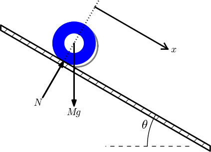
Formulation of physical problems makes heavy use of principal sketches such as the one in Figure 6. This particular sketch illustrates the classical mechanics problem of a rolling wheel on an inclined plane. The figure is made up many individual elements: a rectangle filled with a pattern (the inclined plane), a hollow circle with color (the wheel), arrows with labels (the $ N $ and $ Mg $ forces, and the $ x $ axis), an angle with symbol $ \theta $, and a dashed line indicating the starting location of the wheel.

Drawing software and plotting programs can produce such figures quite easily in principle, but the amount of details the user needs to control with the mouse can be substantial. Software more tailored to producing sketches of this type would work with more convenient abstractions, such as circle, wall, angle, force arrow, axis, and so forth. And as soon we start programming to construct the figure we get a range of other powerful tools at disposal. For example, we can easily translate and rotate parts of the figure and make an animation that illustrates the physics of the problem. Programming as a superior alternative to interactive drawing is the mantra of this section.

Figure 6: Sketch of a physics problem.

Basic construction of sketches

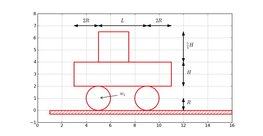
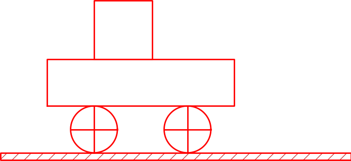
Before attacking real-life sketches as in Figure ref{sketcher:fig1} we focus on the significantly simpler drawing shown in Figure 7. This toy sketch consists of several elements: two circles, two rectangles, and a "ground" element.

Figure 7: Sketch of a simple figure.

Basic drawing

A typical program creating these five elements is shown next. After importing the pysketcher package, the first task is always to define a coordinate system:

from pysketcher import *

drawing_tool.set_coordinate_system(
    xmin=0, xmax=10, ymin=-1, ymax=8)

Instead of working with lengths expressed by specific numbers it is highly recommended to use variables to parameterize lengths as this makes it easier to change dimensions later. Here we introduce some key lengths for the radius of the wheels, distance between the wheels, etc.:

R = 1    # radius of wheel
L = 4    # distance between wheels
H = 2    # height of vehicle body
w_1 = 5  # position of front wheel
drawing_tool.set_coordinate_system(xmin=0, xmax=w_1 + 2*L + 3*R,
                                   ymin=-1, ymax=2*R + 3*H)

With the drawing area in place we can make the first Circle object in an intuitive fashion:

wheel1 = Circle(center=(w_1, R), radius=R)

to change dimensions later.

To translate the geometric information about the wheel1 object to instructions for the plotting engine (in this case Matplotlib), one calls the wheel1.draw(). To display all drawn objects, one issues drawing_tool.display(). The typical steps are hence:

wheel1 = Circle(center=(w_1, R), radius=R)
wheel1.draw()

# Define other objects and call their draw() methods
drawing_tool.display()
drawing_tool.savefig('tmp.png')  # store picture

The next wheel can be made by taking a copy of wheel1 and translating the object to the right according to a displacement vector $ (L,0) $:

wheel2 = wheel1.copy()
wheel2.translate((L,0))

The two rectangles are also made in an intuitive way:

under = Rectangle(lower_left_corner=(w_1-2*R, 2*R),
                  width=2*R + L + 2*R, height=H)
over  = Rectangle(lower_left_corner=(w_1, 2*R + H),
                  width=2.5*R, height=1.25*H)

Groups of objects

Instead of calling the draw method of every object, we can group objects and call draw, or perform other operations, for the whole group. For example, we may collect the two wheels in a wheels group and the over and under rectangles in a body group. The whole vehicle is a composition of its wheels and body groups. The code goes like

wheels  = Composition({'wheel1': wheel1, 'wheel2': wheel2})
body    = Composition({'under': under, 'over': over})

vehicle = Composition({'wheels': wheels, 'body': body})

The ground is illustrated by an object of type Wall, mostly used to indicate walls in sketches of mechanical systems. A Wall takes the x and y coordinates of some curve, and a thickness parameter, and creates a thick curve filled with a simple pattern. In this case the curve is just a flat line so the construction is made of two points on the ground line ($ (w_1-L,0) $ and $ (w_1+3L,0) $):

ground = Wall(x=[w_1 - L, w_1 + 3*L], y=[0, 0], thickness=-0.3*R)

The negative thickness makes the pattern-filled rectangle appear below the defined line, otherwise it appears above.

We may now collect all the objects in a "top" object that contains the whole figure:

fig = Composition({'vehicle': vehicle, 'ground': ground})
fig.draw()  # send all figures to plotting backend
drawing_tool.display()
drawing_tool.savefig('tmp.png')

The fig.draw() call will visit all subgroups, their subgroups, and so forth in the hierarchical tree structure of figure elements, and call draw for every object.

Changing line styles and colors

Controlling the line style, line color, and line width is fundamental when designing figures. The pysketcher package allows the user to control such properties in single objects, but also set global properties that are used if the object has no particular specification of the properties. Setting the global properties are done like

drawing_tool.set_linestyle('dashed')
drawing_tool.set_linecolor('black')
drawing_tool.set_linewidth(4)

At the object level the properties are specified in a similar way:

wheels.set_linestyle('solid')
wheels.set_linecolor('red')

and so on.

Geometric figures can be specified as filled, either with a color or with a special visual pattern:

# Set filling of all curves
drawing_tool.set_filled_curves(color='blue', pattern='/')

# Turn off filling of all curves
drawing_tool.set_filled_curves(False)

# Fill the wheel with red color
wheel1.set_filled_curves('red')

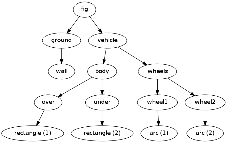
The figure composition as an object hierarchy

The composition of objects making up the figure is hierarchical, similar to a family, where each object has a parent and a number of children. Do a print fig to display the relations:

ground
    wall
vehicle
    body
        over
            rectangle
        under
            rectangle
    wheels
        wheel1
            arc
        wheel2
            arc

The indentation reflects how deep down in the hierarchy (family) we are. This output is to be interpreted as follows:

fig contains two objects, ground and vehicle
ground contains an object wall
vehicle contains two objects, body and wheels
body contains two objects, over and under
wheels contains two objects, wheel1 and wheel2

In this listing there are also objects not defined by the programmer: rectangle and arc. These are of type Curve and automatically generated by the classes Rectangle and Circle.

More detailed information can be printed by

print fig.show_hierarchy('std')

yielding the output

ground (Wall):
    wall (Curve): 4 coords fillcolor='white' fillpattern='/'
vehicle (Composition):
    body (Composition):
        over (Rectangle):
            rectangle (Curve): 5 coords
        under (Rectangle):
            rectangle (Curve): 5 coords
    wheels (Composition):
        wheel1 (Circle):
            arc (Curve): 181 coords
        wheel2 (Circle):
            arc (Curve): 181 coords

Here we can see the class type for each figure object, how many coordinates that are involved in basic figures (Curve objects), and special settings of the basic figure (fillcolor, line types, etc.). For example, wheel2 is a Circle object consisting of an arc, which is a Curve object consisting of 181 coordinates (the points needed to draw a smooth circle). The Curve objects are the only objects that really holds specific coordinates to be drawn. The other object types are just compositions used to group parts of the complete figure.

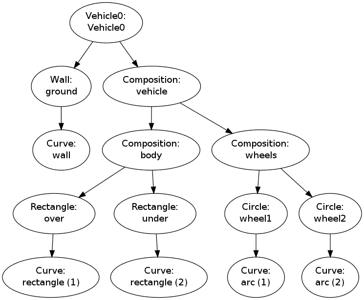
One can also get a graphical overview of the hierarchy of figure objects that build up a particular figure fig. Just call fig.graphviz_dot('fig') to produce a file fig.dot in the dot format. This file contains relations between parent and child objects in the figure and can be turned into an image, as in Figure 8, by running the dot program:

Terminal> dot -Tpng -o fig.png fig.dot

Figure 8: Hierarchical relation between figure objects.

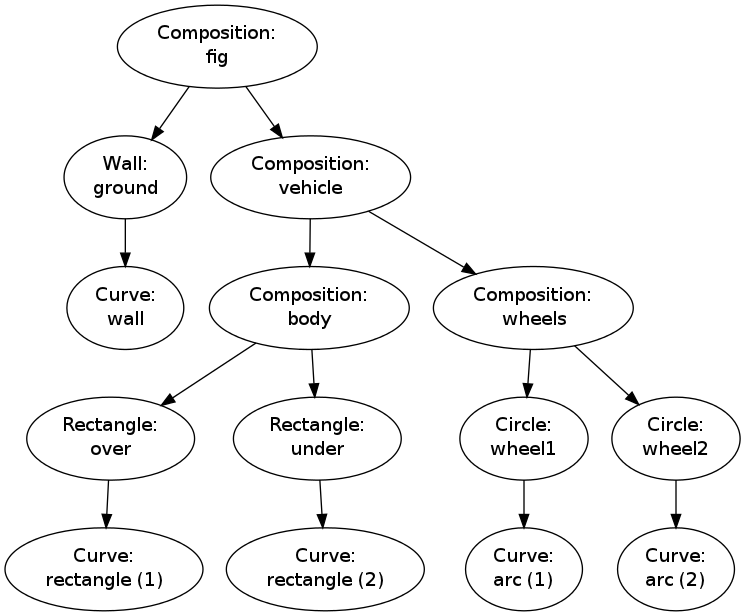
The call fig.graphviz_dot('fig', classname=True) makes a fig.dot file where the class type of each object is also visible, see Figure 9. The ability to write out the object hierarchy or view it graphically can be of great help when working with complex figures that involve layers of subfigures.

Figure 9: Hierarchical relation between figure objects, including their class names.

Any of the objects can in the program be reached through their names, e.g.,

fig['vehicle']
fig['vehicle']['wheels']
fig['vehicle']['wheels']['wheel2']
fig['vehicle']['wheels']['wheel2']['arc']
fig['vehicle']['wheels']['wheel2']['arc'].x  # x coords
fig['vehicle']['wheels']['wheel2']['arc'].y  # y coords
fig['vehicle']['wheels']['wheel2']['arc'].linestyle
fig['vehicle']['wheels']['wheel2']['arc'].linetype

Grabbing a part of the figure this way is handy for changing properties of that part, for example, colors, line styles (see Figure 10):

fig['vehicle']['wheels'].set_filled_curves('blue')
fig['vehicle']['wheels'].set_linewidth(6)
fig['vehicle']['wheels'].set_linecolor('black')

fig['vehicle']['body']['under'].set_filled_curves('red')

fig['vehicle']['body']['over'].set_filled_curves(pattern='/')
fig['vehicle']['body']['over'].set_linewidth(14)
fig['vehicle']['body']['over']['rectangle'].linewidth = 4

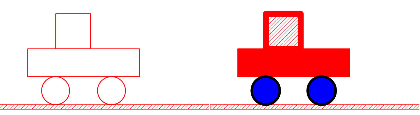
The last line accesses the Curve object directly, while the line above, accesses the Rectangle object, which will then set the linewidth of its Curve object, and other objects if it had any. The result of the actions above is shown in Figure 10.

Figure 10: Left: Basic line-based drawing. Right: Thicker lines and filled parts.

We can also change position of parts of the figure and thereby make animations, as shown next.

Animation: translating the vehicle

Can we make our little vehicle roll? A first attempt will be to fake rolling by just displacing all parts of the vehicle. The relevant parts constitute the fig['vehicle'] object. This part of the figure can be translated, rotated, and scaled. A translation along the ground means a translation in $ x $ direction, say a length $ L $ to the right:

fig['vehicle'].translate((L,0))

You need to erase, draw, and display to see the movement:

drawing_tool.erase()
fig.draw()
drawing_tool.display()

Without erasing, the old drawing of the vehicle will remain in the figure so you get two vehicles. Without fig.draw() the new coordinates of the vehicle will not be communicated to the drawing tool, and without calling display the updated drawing will not be visible.

A figure that moves in time is conveniently realized by the function animate:

animate(fig, tp, action)

Here, fig is the entire figure, tp is an array of time points, and action is a user-specified function that changes fig at a specific time point. Typically, action will move parts of fig.

In the present case we can define the movement through a velocity function v(t) and displace the figure v(t)*dt for small time intervals dt. A possible velocity function is

def v(t):
    return -8*R*t*(1 - t/(2*R))

Our action function for horizontal displacements v(t)*dt becomes

def move(t, fig):
    x_displacement = dt*v(t)
    fig['vehicle'].translate((x_displacement, 0))

Since our velocity is negative for $ t\in [0,2R] $ the displacement is to the left.

The animate function will for each time point t in tp erase the drawing, call action(t, fig), and show the new figure by fig.draw() and drawing_tool.display(). Here we choose a resolution of the animation corresponding to 25 time points in the time interval $ [0,2R] $:

import numpy
tp = numpy.linspace(0, 2*R, 25)
dt = tp[1] - tp[0]  # time step

animate(fig, tp, move, pause_per_frame=0.2)

The pause_per_frame adds a pause, here 0.2 seconds, between each frame in the animation.

We can also ask animate to store each frame in a file:

files = animate(fig, tp, move_vehicle, moviefiles=True,
                pause_per_frame=0.2)

The files variable, here 'tmp_frame_%04d.png', is the printf-specification used to generate the individual plot files. We can use this specification to make a video file via ffmpeg (or avconv on Debian-based Linux systems such as Ubuntu). Videos in the Flash and WebM formats can be created by

Terminal> ffmpeg -r 12 -i tmp_frame_%04d.png -vcodec flv mov.flv
Terminal> ffmpeg -r 12 -i tmp_frame_%04d.png -vcodec libvpx mov.webm

An animated GIF movie can also be made using the convert program from the ImageMagick software suite:

Terminal> convert -delay 20 tmp_frame*.png mov.gif
Terminal> animate mov.gif  # play movie

The delay between frames, in units of 1/100 s, governs the speed of the movie. To play the animated GIF file in a web page, simply insert <img src="mov.gif"> in the HTML code.

The individual PNG frames can be directly played in a web browser by running

Terminal> scitools movie output_file=mov.html fps=5 tmp_frame*

or calling

from scitools.std import movie
movie(files, encoder='html', output_file='mov.html')

in Python. Load the resulting file mov.html into a web browser to play the movie.

Try to run vehicle0.py and then load mov.html into a browser, or play one of the mov.* video files. Alternatively, you can view a ready-made movie.

Animation: rolling the wheels

It is time to show rolling wheels. To this end, we add spokes to the wheels, formed by two crossing lines, see Figure 11. The construction of the wheels will now involve a circle and two lines:

wheel1 = Composition({
    'wheel': Circle(center=(w_1, R), radius=R),
    'cross': Composition({'cross1': Line((w_1,0),   (w_1,2*R)),
                          'cross2': Line((w_1-R,R), (w_1+R,R))})})
wheel2 = wheel1.copy()
wheel2.translate((L,0))

Observe that wheel1.copy() copies all the objects that make up the first wheel, and wheel2.translate translates all the copied objects.

Figure 11: Wheels with spokes to illustrate rolling.

The move function now needs to displace all the objects in the entire vehicle and also rotate the cross1 and cross2 objects in both wheels. The rotation angle follows from the fact that the arc length of a rolling wheel equals the displacement of the center of the wheel, leading to a rotation angle

angle = - x_displacement/R

With w_1 tracking the $ x $ coordinate of the center of the front wheel, we can rotate that wheel by

w1 = fig['vehicle']['wheels']['wheel1']
from math import degrees
w1.rotate(degrees(angle), center=(w_1, R))

The rotate function takes two parameters: the rotation angle (in degrees) and the center point of the rotation, which is the center of the wheel in this case. The other wheel is rotated by

w2 = fig['vehicle']['wheels']['wheel2']
w2.rotate(degrees(angle), center=(w_1 + L, R))

That is, the angle is the same, but the rotation point is different. The update of the center point is done by w_1 += x_displacement. The complete move function with translation of the entire vehicle and rotation of the wheels then becomes

w_1 = w_1 + L   # start position

def move(t, fig):
    x_displacement = dt*v(t)
    fig['vehicle'].translate((x_displacement, 0))

    # Rotate wheels
    global w_1
    w_1 += x_displacement
    # R*angle = -x_displacement
    angle = - x_displacement/R
    w1 = fig['vehicle']['wheels']['wheel1']
    w1.rotate(degrees(angle), center=(w_1, R))
    w2 = fig['vehicle']['wheels']['wheel2']
    w2.rotate(degrees(angle), center=(w_1 + L, R))

The complete example is found in the file vehicle1.py. You may run this file or watch a ready-made movie.

The advantages with making figures this way, through programming rather than using interactive drawing programs, are numerous. For example, the objects are parameterized by variables so that various dimensions can easily be changed. Subparts of the figure, possible involving a lot of figure objects, can change color, linetype, filling or other properties through a single function call. Subparts of the figure can be rotated, translated, or scaled. Subparts of the figure can also be copied and moved to other parts of the drawing area. However, the single most important feature is probably the ability to make animations governed by mathematical formulas or data coming from physics simulations of the problem, as shown in the example above.

Inner workings of the Pysketcher tool

We shall now explain how we can, quite easily, realize software with the capabilities demonstrated in the previous examples. Each object in the figure is represented as a class in a class hierarchy. Using inheritance, classes can inherit properties from parent classes and add new geometric features.

Class programming is a key technology for realizing Pysketcher. As soon as some classes are established, more are easily added. Enhanced functionality for all the classes is also easy to implement in common, generic code that can immediately be shared by all present and future classes. The fundamental data structure involved in the pysketcher package is a hierarchical tree, and much of the material on implementation issues targets how to traverse tree structures with recursive function calls in object hierarchies. This topic is of key relevance in a wide range of other applications as well. In total, the inner workings of Pysketcher constitute an excellent example on the power of class programming.

Example of classes for geometric objects

We introduce class Shape as superclass for all specialized objects in a figure. This class does not store any data, but provides a series of functions that add functionality to all the subclasses. This will be shown later.

Simple geometric objects

One simple subclass is Rectangle, specified by the coordinates of the lower left corner and its width and height:

class Rectangle(Shape):
    def __init__(self, lower_left_corner, width, height):
        p = lower_left_corner  # short form
        x = [p[0], p[0] + width,
             p[0] + width, p[0], p[0]]
        y = [p[1], p[1], p[1] + height,
             p[1] + height, p[1]]
        self.shapes = {'rectangle': Curve(x,y)}

Any subclass of Shape will have a constructor that takes geometric information about the shape of the object and creates a dictionary self.shapes with the shape built of simpler shapes. The most fundamental shape is Curve, which is just a collection of $ (x,y) $ coordinates in two arrays x and y. Drawing the Curve object is a matter of plotting y versus x. For class Rectangle the x and y arrays contain the corner points of the rectangle in counterclockwise direction, starting and ending with in the lower left corner.

Class Line is also a simple class:

class Line(Shape):
    def __init__(self, start, end):
        x = [start[0], end[0]]
        y = [start[1], end[1]]
        self.shapes = {'line': Curve(x, y)}

Here we only need two points, the start and end point on the line. However, we may want to add some useful functionality, e.g., the ability to give an $ x $ coordinate and have the class calculate the corresponding $ y $ coordinate:

    def __call__(self, x):
        """Given x, return y on the line."""
        x, y = self.shapes['line'].x, self.shapes['line'].y
        self.a = (y[1] - y[0])/(x[1] - x[0])
        self.b = y[0] - self.a*x[0]
        return self.a*x + self.b

Unfortunately, this is too simplistic because vertical lines cannot be handled (infinite self.a). The true source code of Line therefore provides a more general solution at the cost of significantly longer code with more tests.

A circle implies a somewhat increased complexity. Again we represent the geometric object by a Curve object, but this time the Curve object needs to store a large number of points on the curve such that a plotting program produces a visually smooth curve. The points on the circle must be calculated manually in the constructor of class Circle. The formulas for points $ (x,y) $ on a curve with radius $ R $ and center at $ (x_0, y_0) $ are given by $$ \begin{align*} x &= x_0 + R\cos (t),\\ y &= y_0 + R\sin (t), \end{align*} $$ where $ t\in [0, 2\pi] $. A discrete set of $ t $ values in this interval gives the corresponding set of $ (x,y) $ coordinates on the circle. The user must specify the resolution as the number of $ t $ values. The circle's radius and center must of course also be specified.

We can write the Circle class as

class Circle(Shape):
    def __init__(self, center, radius, resolution=180):
        self.center, self.radius = center, radius
        self.resolution = resolution

        t = linspace(0, 2*pi, resolution+1)
        x0 = center[0];  y0 = center[1]
        R = radius
        x = x0 + R*cos(t)
        y = y0 + R*sin(t)
        self.shapes = {'circle': Curve(x, y)}

As in class Line we can offer the possibility to give an angle $ \theta $ (equivalent to $ t $ in the formulas above) and then get the corresponding $ x $ and $ y $ coordinates:

    def __call__(self, theta):
        """Return (x, y) point corresponding to angle theta."""
        return self.center[0] + self.radius*cos(theta), \ 
               self.center[1] + self.radius*sin(theta)

There is one flaw with this method: it yields illegal values after a translation, scaling, or rotation of the circle.

A part of a circle, an arc, is a frequent geometric object when drawing mechanical systems. The arc is constructed much like a circle, but $ t $ runs in $ [\theta_s, \theta_s + \theta_a] $. Giving $ \theta_s $ and $ \theta_a $ the slightly more descriptive names start_angle and arc_angle, the code looks like this:

class Arc(Shape):
    def __init__(self, center, radius,
                 start_angle, arc_angle,
                 resolution=180):
        self.start_angle = radians(start_angle)
        self.arc_angle = radians(arc_angle)

        t = linspace(self.start_angle,
                     self.start_angle + self.arc_angle,
                     resolution+1)
        x0 = center[0];  y0 = center[1]
        R = radius
        x = x0 + R*cos(t)
        y = y0 + R*sin(t)
        self.shapes = {'arc': Curve(x, y)}

Having the Arc class, a Circle can alternatively be defined as a subclass specializing the arc to a circle:

class Circle(Arc):
    def __init__(self, center, radius, resolution=180):
        Arc.__init__(self, center, radius, 0, 360, resolution)

Class curve

Class Curve sits on the coordinates to be drawn, but how is that done? The constructor of class Curve just stores the coordinates, while a method draw sends the coordinates to the plotting program to make a graph. Or more precisely, to avoid a lot of (e.g.) Matplotlib-specific plotting commands in class Curve we have created a small layer with a simple programming interface to plotting programs. This makes it straightforward to change from Matplotlib to another plotting program. The programming interface is represented by the drawing_tool object and has a few functions:

plot_curve for sending a curve in terms of $ x $ and $ y $ coordinates to the plotting program,
set_coordinate_system for specifying the graphics area,
erase for deleting all elements of the graph,
set_grid for turning on a grid (convenient while constructing the figure),
set_instruction_file for creating a separate file with all plotting commands (Matplotlib commands in our case),
a series of set_X functions where X is some property like linecolor, linestyle, linewidth, filled_curves.

This is basically all we need to communicate to a plotting program.

Any class in the Shape hierarchy inherits set_X functions for setting properties of curves. This information is propagated to all other shape objects in the self.shapes dictionary. Class Curve stores the line properties together with the coordinates of its curve and propagates this information to the plotting program. When saying vehicle.set_linewidth(10), all objects that make up the vehicle object will get a set_linewidth(10) call, but only the Curve object at the end of the chain will actually store the information and send it to the plotting program.

A rough sketch of class Curve reads

class Curve(Shape):
    """General curve as a sequence of (x,y) coordintes."""
    def __init__(self, x, y):
        self.x = asarray(x, dtype=float)
        self.y = asarray(y, dtype=float)

    def draw(self):
        drawing_tool.plot_curve(
            self.x, self.y,
            self.linestyle, self.linewidth, self.linecolor, ...)

    def set_linewidth(self, width):
        self.linewidth = width

    det set_linestyle(self, style):
        self.linestyle = style
    ...

Compound geometric objects

The simple classes Line, Arc, and Circle could can the geometric shape through just one Curve object. More complicated shapes are built from instances of various subclasses of Shape. Classes used for professional drawings soon get quite complex in composition and have a lot of geometric details, so here we prefer to make a very simple composition: the already drawn vehicle from Figure 7. That is, instead of composing the drawing in a Python program as shown above, we make a subclass Vehicle0 in the Shape hierarchy for doing the same thing.

The Shape hierarchy is found in the pysketcher package, so to use these classes or derive a new one, we need to import pysketcher. The constructor of class Vehicle0 performs approximately the same statements as in the example program we developed for making the drawing in Figure 7.

from pysketcher import *

class Vehicle0(Shape):
    def __init__(self, w_1, R, L, H):
        wheel1 = Circle(center=(w_1, R), radius=R)
        wheel2 = wheel1.copy()
        wheel2.translate((L,0))

        under = Rectangle(lower_left_corner=(w_1-2*R, 2*R),
                          width=2*R + L + 2*R, height=H)
        over  = Rectangle(lower_left_corner=(w_1, 2*R + H),
                          width=2.5*R, height=1.25*H)

        wheels = Composition(
            {'wheel1': wheel1, 'wheel2': wheel2})
        body = Composition(
            {'under': under, 'over': over})

        vehicle = Composition({'wheels': wheels, 'body': body})
        xmax = w_1 + 2*L + 3*R
        ground = Wall(x=[R, xmax], y=[0, 0], thickness=-0.3*R)

        self.shapes = {'vehicle': vehicle, 'ground': ground}

Any subclass of Shape must define the shapes attribute, otherwise the inherited draw method (and a lot of other methods too) will not work.

The painting of the vehicle, as shown in the right part of Figure 10, could in class Vehicle0 be offered by a method:

    def colorful(self):
        wheels = self.shapes['vehicle']['wheels']
        wheels.set_filled_curves('blue')
        wheels.set_linewidth(6)
        wheels.set_linecolor('black')
        under = self.shapes['vehicle']['body']['under']
        under.set_filled_curves('red')
        over = self.shapes['vehicle']['body']['over']
        over.set_filled_curves(pattern='/')
        over.set_linewidth(14)

The usage of the class is simple: after having set up an appropriate coordinate system as previously shown, we can do

vehicle = Vehicle0(w_1, R, L, H)
vehicle.draw()
drawing_tool.display()

and go on the make a painted version by

drawing_tool.erase()
vehicle.colorful()
vehicle.draw()
drawing_tool.display()

A complete code defining and using class Vehicle0 is found in the file vehicle2.py.

The pysketcher package contains a wide range of classes for various geometrical objects, particularly those that are frequently used in drawings of mechanical systems.

Adding functionality via recursion

The really powerful feature of our class hierarchy is that we can add much functionality to the superclass Shape and to the "bottom" class Curve, and then all other classes for various types of geometrical shapes immediately get the new functionality. To explain the idea we may look at the draw method, which all classes in the Shape hierarchy must have. The inner workings of the draw method explain the secrets of how a series of other useful operations on figures can be implemented.

Basic principles of recursion

Note that we work with two types of hierarchies in the present documentation: one Python class hierarchy, with Shape as superclass, and one object hierarchy of figure elements in a specific figure. A subclass of Shape stores its figure in the self.shapes dictionary. This dictionary represents the object hierarchy of figure elements for that class. We want to make one draw call for an instance, say our class Vehicle0, and then we want this call to be propagated to all objects that are contained in self.shapes and all is nested subdictionaries. How is this done?

The natural starting point is to call draw for each Shape object in the self.shapes dictionary:

def draw(self):
    for shape in self.shapes:
        self.shapes[shape].draw()

This general method can be provided by class Shape and inherited in subclasses like Vehicle0. Let v be a Vehicle0 instance. Seemingly, a call v.draw() just calls

v.shapes['vehicle'].draw()
v.shapes['ground'].draw()

However, in the former call we call the draw method of a Composition object whose self.shapes attributed has two elements: wheels and body. Since class Composition inherits the same draw method, this method will run through self.shapes and call wheels.draw() and body.draw(). Now, the wheels object is also a Composition with the same draw method, which will run through self.shapes, now containing the wheel1 and wheel2 objects. The wheel1 object is a Circle, so calling wheel1.draw() calls the draw method in class Circle, but this is the same draw method as shown above. This method will therefore traverse the circle's shapes dictionary, which we have seen consists of one Curve element.

The Curve object holds the coordinates to be plotted so here draw really needs to do something "physical", namely send the coordinates to the plotting program. The draw method is outlined in the short listing of class Curve shown previously.

We can go to any of the other shape objects that appear in the figure hierarchy and follow their draw calls in the similar way. Every time, a draw call will invoke a new draw call, until we eventually hit a Curve object at the "bottom" of the figure hierarchy, and then that part of the figure is really plotted (or more precisely, the coordinates are sent to a plotting program).

When a method calls itself, such as draw does, the calls are known as recursive and the programming principle is referred to as recursion. This technique is very often used to traverse hierarchical structures like the figure structures we work with here. Even though the hierarchy of objects building up a figure are of different types, they all inherit the same draw method and therefore exhibit the same behavior with respect to drawing. Only the Curve object has a different draw method, which does not lead to more recursion.

Explaining recursion

Understanding recursion is usually a challenge. To get a better idea of how recursion works, we have equipped class Shape with a method recurse that just visits all the objects in the shapes dictionary and prints out a message for each object. This feature allows us to trace the execution and see exactly where we are in the hierarchy and which objects that are visited.

The recurse method is very similar to draw:

    def recurse(self, name, indent=0):
        # print message where we are (name is where we come from)
        for shape in self.shapes:
            # print message about which object to visit
            self.shapes[shape].recurse(indent+2, shape)

The indent parameter governs how much the message from this recurse method is intended. We increase indent by 2 for every level in the hierarchy, i.e., every row of objects in Figure 12. This indentation makes it easy to see on the printout how far down in the hierarchy we are.

A typical message written by recurse when name is 'body' and the shapes dictionary has the keys 'over' and 'under', will be

     Composition: body.shapes has entries 'over', 'under'
     call body.shapes["over"].recurse("over", 6)

The number of leading blanks on each line corresponds to the value of indent. The code printing out such messages looks like

    def recurse(self, name, indent=0):
        space = ' '*indent
        print space, '%s: %s.shapes has entries' % \ 
              (self.__class__.__name__, name), \ 
              str(list(self.shapes.keys()))[1:-1]

        for shape in self.shapes:
            print space,
            print 'call %s.shapes["%s"].recurse("%s", %d)' % \ 
                  (name, shape, shape, indent+2)
            self.shapes[shape].recurse(shape, indent+2)

Let us follow a v.recurse('vehicle') call in detail, v being a Vehicle0 instance. Before looking into the output from recurse, let us get an overview of the figure hierarchy in the v object (as produced by print v)

ground
    wall
vehicle
    body
        over
            rectangle
        under
            rectangle
    wheels
        wheel1
            arc
        wheel2
            arc

The recurse method performs the same kind of traversal of the hierarchy, but writes out and explains a lot more.

The data structure represented by v.shapes is known as a tree. As in physical trees, there is a root, here the v.shapes dictionary. A graphical illustration of the tree (upside down) is shown in Figure 12. From the root there are one or more branches, here two: ground and vehicle. Following the vehicle branch, it has two new branches, body and wheels. Relationships as in family trees are often used to describe the relations in object trees too: we say that vehicle is the parent of body and that body is a child of vehicle. The term node is also often used to describe an element in a tree. A node may have several other nodes as descendants.

Figure 12: Hierarchy of figure elements in an instance of class Vehicle0.

Recursion is the principal programming technique to traverse tree structures. Any object in the tree can be viewed as a root of a subtree. For example, wheels is the root of a subtree that branches into wheel1 and wheel2. So when processing an object in the tree, we imagine we process the root and then recurse into a subtree, but the first object we recurse into can be viewed as the root of the subtree, so the processing procedure of the parent object can be repeated.

A recommended next step is to simulate the recurse method by hand and carefully check that what happens in the visits to recurse is consistent with the output listed below. Although tedious, this is a major exercise that guaranteed will help to demystify recursion.

A part of the printout of v.recurse('vehicle') looks like

 Vehicle0: vehicle.shapes has entries 'ground', 'vehicle'
 call vehicle.shapes["ground"].recurse("ground", 2)
   Wall: ground.shapes has entries 'wall'
   call ground.shapes["wall"].recurse("wall", 4)
     reached "bottom" object Curve
 call vehicle.shapes["vehicle"].recurse("vehicle", 2)
   Composition: vehicle.shapes has entries 'body', 'wheels'
   call vehicle.shapes["body"].recurse("body", 4)
     Composition: body.shapes has entries 'over', 'under'
     call body.shapes["over"].recurse("over", 6)
       Rectangle: over.shapes has entries 'rectangle'
       call over.shapes["rectangle"].recurse("rectangle", 8)
         reached "bottom" object Curve
     call body.shapes["under"].recurse("under", 6)
       Rectangle: under.shapes has entries 'rectangle'
       call under.shapes["rectangle"].recurse("rectangle", 8)
         reached "bottom" object Curve
...

This example should clearly demonstrate the principle that we can start at any object in the tree and do a recursive set of calls with that object as root.

Scaling, translating, and rotating a figure

With recursion, as explained in the previous section, we can within minutes equip all classes in the Shape hierarchy, both present and future ones, with the ability to scale the figure, translate it, or rotate it. This added functionality requires only a few lines of code.

Scaling

We start with the simplest of the three geometric transformations, namely scaling. For a Curve instance containing a set of $ n $ coordinates $ (x_i,y_i) $ that make up a curve, scaling by a factor $ a $ means that we multiply all the $ x $ and $ y $ coordinates by $ a $: $$ x_i \leftarrow ax_i,\quad y_i\leftarrow ay_i, \quad i=0,\ldots,n-1\thinspace . $$ Here we apply the arrow as an assignment operator. The corresponding Python implementation in class Curve reads

class Curve:
    ...
    def scale(self, factor):
        self.x = factor*self.x
        self.y = factor*self.y

Note here that self.x and self.y are Numerical Python arrays, so that multiplication by a scalar number factor is a vectorized operation.

An even more efficient implementation is to make use of in-place multiplication in the arrays,

class Curve:
    ...
    def scale(self, factor):
        self.x *= factor
        self.y *= factor

as this saves the creation of temporary arrays like factor*self.x.

In an instance of a subclass of Shape, the meaning of a method scale is to run through all objects in the dictionary shapes and ask each object to scale itself. This is the same delegation of actions to subclass instances as we do in the draw (or recurse) method. All objects, except Curve instances, can share the same implementation of the scale method. Therefore, we place the scale method in the superclass Shape such that all subclasses inherit the method. Since scale and draw are so similar, we can easily implement the scale method in class Shape by copying and editing the draw method:

class Shape:
    ...
    def scale(self, factor):
        for shape in self.shapes:
            self.shapes[shape].scale(factor)

This is all we have to do in order to equip all subclasses of Shape with scaling functionality! Any piece of the figure will scale itself, in the same manner as it can draw itself.

Translation

A set of coordinates $ (x_i, y_i) $ can be translated $ v_0 $ units in the $ x $ direction and $ v_1 $ units in the $ y $ direction using the formulas $$ \begin{equation*} x_i\leftarrow x_i+v_0,\quad y_i\leftarrow y_i+v_1, \quad i=0,\ldots,n-1\thinspace . \end{equation*} $$ The natural specification of the translation is in terms of the vector $ v=(v_0,v_1) $. The corresponding Python implementation in class Curve becomes

class Curve:
    ...
    def translate(self, v):
        self.x += v[0]
        self.y += v[1]

The translation operation for a shape object is very similar to the scaling and drawing operations. This means that we can implement a common method translate in the superclass Shape. The code is parallel to the scale method:

class Shape:
    ....
    def translate(self, v):
        for shape in self.shapes:
            self.shapes[shape].translate(v)

Rotation

Rotating a figure is more complicated than scaling and translating. A counter clockwise rotation of $ \theta $ degrees for a set of coordinates $ (x_i,y_i) $ is given by $$ \begin{align*} \bar x_i &\leftarrow x_i\cos\theta - y_i\sin\theta,\\ \bar y_i &\leftarrow x_i\sin\theta + y_i\cos\theta\thinspace . \end{align*} $$ This rotation is performed around the origin. If we want the figure to be rotated with respect to a general point $ (x,y) $, we need to extend the formulas above: $$ \begin{align*} \bar x_i &\leftarrow x + (x_i -x)\cos\theta - (y_i -y)\sin\theta,\\ \bar y_i &\leftarrow y + (x_i -x)\sin\theta + (y_i -y)\cos\theta\thinspace . \end{align*} $$ The Python implementation in class Curve, assuming that $ \theta $ is given in degrees and not in radians, becomes

    def rotate(self, angle, center):
        angle = radians(angle)
        x, y = center
        c = cos(angle);  s = sin(angle)
        xnew = x + (self.x - x)*c - (self.y - y)*s
        ynew = y + (self.x - x)*s + (self.y - y)*c
        self.x = xnew
        self.y = ynew

The rotate method in class Shape follows the principle of the draw, scale, and translate methods.

We have already seen the rotate method in action when animating the rolling wheel at the end of the section Animation: rolling the wheels.

Classes for DNA analysis

We shall here exemplify the use of classes for performing DNA analysis as explained in the previous text. Basically, we create a class Gene to represent a DNA sequence (string) and a class Region to represent a subsequence (substring), typically an exon or intron.

Class for regions

The class for representing a region of a DNA string is quite simple:

class Region(object):
    def __init__(self, dna, start, end):
        self._region = dna[start:end]

    def get_region(self):
        return self._region

    def __len__(self):
        return len(self._region)

    def __eq__(self, other):
        """Check if two Region instances are equal."""
        return self._region == other._region

    def __add__(self, other):
        """Add Region instances: self + other"""
        return self._region + other._region

    def __iadd__(self, other):
        """Increment Region instance: self += other"""
        self._region += other._region
        return self

Besides storing the substring and giving access to it through get_region, we have also included the possibility to

say len(r) if r is a Region instance
check if two Region instances are equal
write r1 + r2 for two instances r1 and r2 of type Region
perform r1 += r2

The latter two operations are convenient for making one large string out of all exon or intron regions.

Class for genes

The class for gene will be longer and more complex than class Region. We already have a bunch of functions performing various types of analysis. The idea of the Gene class is that these functions are methods in the class operating on the DNA string and the exon regions stored in the class. Rather than recoding all the functions as methods in the class we shall just let the class "wrap" the functions. That is, the class methods call up the functions we already have. This approach has two advantages: users can either choose the function-based or the class-based interface, and the programmer can reuse all the ready-made functions when implementing the class-based interface.

The selection of functions include

generate_string for generating a random string from some alphabet
download and read_dnafile (version read_dnafile_v1) for downloading data from the Internet and reading from file
read_exon_regions (version read_exon_regions_v2) for reading exon regions from file
tofile_with_line_sep (version tofile_with_line_sep_v2) for writing strings to file
read_genetic_code (version read_genetic_code_v2) for loading the mapping from triplet codes to 1-letter symbols for amino acids
get_base_frequencies (version get_base_frequencies_v2) for finding frequencies of each base
format_frequencies for formatting base frequencies with two decimals
create_mRNA for computing an mRNA string from DNA and exon regions
mutate for mutating a base at a random position
create_markov_chain, transition, and mutate_via_markov_chain for mutating a base at a random position according to randomly generated transition probabilities
create_protein_fixed for proper creation of a protein sequence (string)

The set of plain functions for DNA analysis is found in the file dna_functions.py, while dna_classes.py contains the implementations of classes Gene and Region.

Basic features of class gene

Class Gene is supposed to hold the DNA sequence and the associated exon regions. A simple constructor expects the exon regions to be specified as a list of (start, end) tuples indicating the start and end of each region:

class Gene(object):
    def __init__(self, dna, exon_regions):
        self._dna = dna

        self._exon_regions = exon_regions
        self._exons = []
        for start, end in exon_regions:
            self._exons.append(Region(dna, start, end))

        # Compute the introns (regions between the exons)
        self._introns = []
        prev_end = 0
        for start, end in exon_regions:
            self._introns.append(Region(dna, prev_end, start))
            prev_end = end
        self._introns.append(Region(dna, end, len(dna)))

The methods in class Gene are trivial to implement when we already have the functionality in stand-alone functions. Here are a few examples on methods:

from dna_functions import *

class Gene(object):
    ...

    def write(self, filename, chars_per_line=70):
        """Write DNA sequence to file with name filename."""
        tofile_with_line_sep(self._dna, filename, chars_per_line)

    def count(self, base):
        """Return no of occurrences of base in DNA."""
        return self._dna.count(base)

    def get_base_frequencies(self):
        """Return dict of base frequencies in DNA."""
        return get_base_frequencies(self._dna)

    def format_base_frequencies(self):
        """Return base frequencies formatted with two decimals."""
        return format_frequencies(self.get_base_frequencies())

Flexible constructor

The constructor can be made more flexible. First, the exon regions may not be known so we should allow None as value and in fact use that as default value. Second, exon regions at the start and/or end of the DNA string will lead to empty intron Region objects so a proper test on nonzero length of the introns must be inserted. Third, the data for the DNA string and the exon regions can either be passed as arguments or downloaded and read from file. Two different initializations of Gene objects are therefore

g1 = Gene(dna, exon_regions)  # user has read data from file
g2 = Gene((urlbase, dna_file), (urlbase, exon_file))  # download

One can pass None for urlbase if the files are already at the computer. The flexible constructor has, not surprisingly, much longer code than the first version. The implementation illustrates well how the concept of overloaded constructors in other languages, like C++ and Java, are dealt with in Python (overloaded constructors take different types of arguments to initialize an instance):

class Gene(object):
    def __init__(self, dna, exon_regions):
        """
        dna: string or (urlbase,filename) tuple
        exon_regions: None, list of (start,end) tuples
                      or (urlbase,filename) tuple
        In case of (urlbase,filename) tuple the file
        is downloaded and read.
        """
        if isinstance(dna, (list,tuple)) and \ 
           len(dna) == 2 and isinstance(dna[0], str) and \ 
           isinstance(dna[1], str):
            download(urlbase=dna[0], filename=dna[1])
            dna = read_dnafile(dna[1])
        elif isinstance(dna, str):
            pass # ok type (the other possibility)
        else:
            raise TypeError(
                'dna=%s %s is not string or (urlbase,filename) '\ 
                'tuple' % (dna, type(dna)))

        self._dna = dna

        er = exon_regions
        if er is None:
            self._exons = None
            self._introns = None
        else:
            if isinstance(er, (list,tuple)) and \ 
                len(er) == 2 and isinstance(er[0], str) and \ 
                isinstance(er[1], str):
                download(urlbase=er[0], filename=er[1])
                exon_regions = read_exon_regions(er[1])
            elif isinstance(er, (list,tuple)) and \ 
                isinstance(er[0], (list,tuple)) and \ 
                isinstance(er[0][0], int) and \ 
                isinstance(er[0][1], int):
                pass # ok type (the other possibility)
            else:
                raise TypeError(
                    'exon_regions=%s %s is not list of (int,int) '
                    'or (urlbase,filename) tuple' % (er, type(era)))

            self._exon_regions = exon_regions
            self._exons = []
            for start, end in exon_regions:
                self._exons.append(Region(dna, start, end))

            # Compute the introns (regions between the exons)
            self._introns = []
            prev_end = 0
            for start, end in exon_regions:
                if start - prev_end > 0:
                    self._introns.append(
                        Region(dna, prev_end, start))
                prev_end = end
            if len(dna) - end > 0:
                self._introns.append(Region(dna, end, len(dna)))

Note that we perform quite detailed testing of the object type of the data structures supplied as the dna and exon_regions arguments. This can well be done to ensure safe use also when there is only one allowed type per argument.

Other methods

A create_mRNA method, returning the mRNA as a string, can be coded as

    def create_mRNA(self):
        """Return string for mRNA."""
        if self._exons is not None:
            return create_mRNA(self._dna, self._exon_regions)
        else:
            raise ValueError(
                'Cannot create mRNA for gene with no exon regions')

Also here we rely on calling an already implemented function, but include some testing whether asking for mRNA is appropriate.

Methods for creating a mutated gene are also included:

    def mutate_pos(self, pos, base):
        """Return Gene with a mutation to base at position pos."""
        dna = self._dna[:pos] + base + self._dna[pos+1:]
        return Gene(dna, self._exon_regions)

    def mutate_random(self, n=1):
        """
        Return Gene with n mutations at a random position.
        All mutations are equally probable.
        """
        mutated_dna = self._dna
        for i in range(n):
            mutated_dna = mutate(mutated_dna)
        return Gene(mutated_dna, self._exon_regions)

    def mutate_via_markov_chain(markov_chain):
        """
        Return Gene with a mutation at a random position.
        Mutation into new base based on transition
        probabilities in the markov_chain dict of dicts.
        """
        mutated_dna = mutate_via_markov_chain(
            self._dna, markov_chain)
        return Gene(mutated_dna, self._exon_regions)

Some "get" methods that give access to the fundamental attributes of the class can be included:

    def get_dna(self):
        return self._dna

    def get_exons(self):
        return self._exons

    def get_introns(self):
        return self._introns

Alternatively, one could access the attributes directly: gene._dna, gene._exons, etc. In that case we should remove the leading underscore as this underscore signals that these attributes are considered "protected", i.e., not to be directly accessed by the user. The "protection" in "get" functions is more mental than actual since we anyway give the data structures in the hands of the user and she can do whatever she wants (even delete them).

Special methods for the length of a gene, adding genes, checking if two genes are identical, and printing of compact gene information are relevant to add:

    def __len__(self):
        return len(self._dna)

    def __add__(self, other):
        """self + other: append other to self (DNA string)."""
        if self._exons is None and other._exons is None:
            return Gene(self._dna + other._dna, None)
        else:
            raise ValueError(
                'cannot do Gene + Gene with exon regions')

    def __iadd__(self, other):
        """self += other: append other to self (DNA string)."""
        if self._exons is None and other._exons is None:
            self._dna += other._dna
            return self
        else:
            raise ValueError(
                'cannot do Gene += Gene with exon regions')

    def __eq__(self, other):
        """Check if two Gene instances are equal."""
        return self._dna == other._dna and \ 
               self._exons == other._exons

    def __str__(self):
        """Pretty print (condensed info)."""
        s = 'Gene: ' + self._dna[:6] + '...' + self._dna[-6:] + \ 
            ', length=%d' % len(self._dna)
        if self._exons is not None:
            s += ', %d exon regions' % len(self._exons)
        return s

Here is an interactive session demonstrating how we can work with class Gene objects:

>>> from dna_classes import Gene
>>> g1 = Gene('ATCCGTAATTGCGCA', [(2,4), (6,9)])
>>> print g1
Gene: ATCCGT...TGCGCA, length=15, 2 exon regions
>>> g2 = g1.mutate_random(10)
>>> print g2
Gene: ATCCGT...TGTGCT, length=15, 2 exon regions
>>> g1 == g2
False
>>> g1 += g2  # expect exception
Traceback (most recent call last):
...
ValueError: cannot do Gene += Gene with exon regions
>>> g1b = Gene(g1.get_dna(), None)
>>> g2b = Gene(g2.get_dna(), None)
>>> print g1b
Gene: ATCCGT...TGCGCA, length=15
>>> g3 = g1b + g2b
>>> g3.format_base_frequencies()
'A: 0.17, C: 0.23, T: 0.33, G: 0.27'

Subclasses

There are two fundamental types of genes: the most common type that codes for proteins (indirectly via mRNA) and the type that only codes for RNA (without being further processed to proteins). The product of a gene, mRNA or protein, depends on the type of gene we have. It is then natural to create two subclasses for the two types of gene and have a method get_product which returns the product of that type of gene.

The get_product method can be declared in class Gene:

    def get_product(self):
        raise NotImplementedError(
            'Subclass %s must implement get_product' % \ 
            self.__class__.__name__)

The exception here will be triggered by an instance (self) of any subclass that just inherits get_product from class Gene without implementing a subclass version of this method.

The two subclasses of Gene may take this simple form:

class RNACodingGene(Gene):
    def get_product(self):
        return self.create_mRNA()

class ProteinCodingGene(Gene):
    def __init__(self, dna, exon_positions):
        Gene.__init__(self, dna, exon_positions)
        urlbase = 'http://hplgit.github.com/bioinf-py/data/'
        genetic_code_file = 'genetic_code.tsv'
        download(urlbase, genetic_code_file)
        code = read_genetic_code(genetic_code_file)
        self.genetic_code = code

    def get_product(self):
        return create_protein_fixed(self.create_mRNA(),
                                    self.genetic_code)

A demonstration of how to load the lactase gene and create the lactase protein is done with

def test_lactase_gene():
    urlbase = 'http://hplgit.github.com/bioinf-py/data/'
    lactase_gene_file = 'lactase_gene.txt'
    lactase_exon_file = 'lactase_exon.tsv'
    lactase_gene = ProteinCodingGene(
        (urlbase, lactase_gene_file),
        (urlbase, lactase_exon_file))

    protein = lactase_gene.get_product()
    tofile_with_line_sep(protein, 'output', 'lactase_protein.txt')

Now, envision that the Lactase gene would instead have been an RNA-coding gene. The only necessary changes would have been to exchange ProteinCodingGene by RNACodingGene in the assignment to lactase_gene, and one would get out a final RNA product instead of a protein.