This chapter is taken from the book A Primer on Scientific Programming with Python by H. P. Langtangen, 5th edition, Springer, 2016.
Class hierarchy for numerical integration
There are many different numerical methods for integrating a mathematical function, just as there are many different methods for differentiating a function. It is thus obvious that the idea of object-oriented programming and class hierarchies can be applied to numerical integration formulas in the same manner as we did in the section Class hierarchy for numerical differentiation.
Numerical integration methods
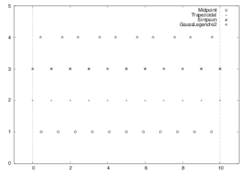
First, we list some different methods for integrating \( \int_a^bf(x)dx \) using \( n \) evaluation points. All the methods can be written as $$ \begin{equation} \int_a^b f(x)dx \approx \sum_{i=0}^{n-1} w_i f(x_i), \tag{8} \end{equation} $$ where \( w_i \) are weights and \( x_i \) are evaluation points, \( i=0,\ldots,n-1 \). The Midpoint method has $$ \begin{equation} x_i = a + {h\over 2} + ih,\quad w_i=h,\quad h={b-a\over n},\quad i=0,\ldots,n-1\tp \tag{9} \end{equation} $$ The Trapezoidal method has the points $$ \begin{equation} x_i = a+ih, \quad h={b-a\over n-1},\quad i=0,\ldots,n-1, \tag{10} \end{equation} $$ and the weights $$ \begin{equation} w_0=w_{n-1}={h\over2},\ w_i=h, \quad i=1,\ldots,n-2\tp \tag{11} \end{equation} $$ Simpson's rule has the same evaluation points as the Trapezoidal rule, but $$ \begin{equation} h = 2{b-a\over n-1},\quad w_0=w_{n-1}={h\over6}, \tag{12} \end{equation} $$ $$ \begin{equation} w_i={h\over3}\hbox{ for } i=2,4,\ldots,n-3, \tag{13} \end{equation} $$ $$ \begin{equation} w_i={2h\over3}\hbox{ for } i=1,3,5,\ldots,n-2\tp \tag{14} \end{equation} $$ Note that \( n \) must be odd in Simpson's rule. A Two-Point Gauss-Legendre method takes the form $$ \begin{equation} x_i = a+(i+ \frac{1}{2})h - {1\over\sqrt{3}}{h\over2}\quad\hbox{for } i=0,2,4,\ldots,n-2, \tag{15} \end{equation} $$ $$ \begin{equation} x_i = a+(i+ \frac{1}{2})h + {1\over\sqrt{3}}{h\over2}\quad\hbox{for } i=1,3,5,\ldots,n-1, \tag{16} \end{equation} $$ with \( h=2(b-a)/n \). Here \( n \) must be even. All the weights have the same value: \( w_i=h/2 \), \( i=0,\ldots,n-1 \). Figure 3 illustrates how the points in various integration rules are distributed over a few intervals.
Figure 3: Illustration of the distribution of points for various numerical integration methods. The Gauss-Legendre method has 10 points, while the other methods have 11 points in \( [0,10] \).
Classes for integration
We may store \( x_i \) and \( w_i \) in two NumPy arrays and compute the integral as \( \sum_{i=0}^{n-1} w_if(x_i) \). This operation can also be vectorized as a dot (inner) product between the \( w_i \) vector and the \( f(x_i) \) vector, provided \( f(x) \) is implemented in a vectorizable form.
We argued in the section ref{sec:class:autoint} that it pays off to implement a numerical integration formula as a class. If we do so with the different methods from the previous section, a typical class looks like this:
class SomeIntegrationMethod(object):
    def __init__(self, a, b, n):
        # Compute self.points and self.weights

    def integrate(self, f):
        s = 0
        for i in range(len(self.weights)):
            s += self.weights[i]*f(self.points[i])
        return s
Making such classes for many different integration methods soon
reveals that all the classes contain common code, namely the
integrate method for computing \( \sum_{i=0}^{n-1} w_if(x_i) \).
Therefore, this common code can be placed in a superclass, and
subclasses can just add the code that is specific to a certain
numerical integration formula, namely the definition of the weights
\( w_i \) and the points \( x_i \).
Let us start with the superclass:
class Integrator(object):
    def __init__(self, a, b, n):
        self.a, self.b, self.n = a, b, n
        self.points, self.weights = self.construct_method()

    def construct_method(self):
        raise NotImplementedError('no rule in class %s' %
                                  self.__class__.__name__)

    def integrate(self, f):
        s = 0
        for i in range(len(self.weights)):
            s += self.weights[i]*f(self.points[i])
        return s
As we have seen, we store the \( a \), \( b \), and \( n \) data about the
integration method in the constructor. Moreover, we compute arrays or
lists self.points for the \( x_i \) points and self.weights for the
\( w_i \) weights. All this code can now be inherited by all subclasses.
The initialization of points and weights is put in a separate method,
construct_method, which is supposed to be implemented in each
subclass, but the superclass provides a default implementation, which
tells the user that the method is not implemented. What happens is
that when subclasses redefine a method, that method overrides the
method inherited from the superclass. Hence, if we forget to redefine
construct_method in a subclass, we will inherit the one from the
superclass, and this method issues an error message. The construction
of this error message is quite clever in the sense that it will tell
in which class the construct_method method is missing (self will
be the subclass instance and its __class__.__name__ is a string with
the corresponding subclass name).
In computer science one usually speaks about overloading a method in a subclass, but the words redefining and overriding are also used. A method that is overloaded is said to be polymorphic. A related term, polymorphism, refers to coding with polymorphic methods. Very often, a superclass provides some default implementation of a method, and a subclass overloads the method with the purpose of tailoring the method to a particular application.
The integrate method is common for all integration rules, i.e., for
all subclasses, so it can be inherited as it is. A vectorized version
can also be added in the superclass to make it automatically available
also in all subclasses:
    def vectorized_integrate(self, f):
        return np.dot(self.weights, f(self.points))
Let us then implement a subclass. Only the construct_method method
needs to be written. For the Midpoint rule, this is a matter of
translating the formulas in (9) to Python:
class Midpoint(Integrator):
    def construct_method(self):
        a, b, n = self.a, self.b, self.n  # quick forms
        h = (b-a)/float(n)
        x = np.linspace(a + 0.5*h, b - 0.5*h, n)
        w = np.zeros(len(x)) + h
        return x, w
Observe that we implemented directly a vectorized code. We could also have used (slow) loops and explicit indexing:
        x = np.zeros(n)
        w = np.zeros(n)
        for i in range(n):
            x[i] = a + 0.5*h + i*h
            w[i] = h
Before we continue with other subclasses for other numerical
integration formulas, we will have a look at the program flow when we
use class Midpoint. Suppose we want to integrate \( \int_0^2x^2dx \)
using \( 101 \) points:
def f(x): return x*x
m = Midpoint(0, 2, 101)
print m.integrate(f)
How is the program flow? The assignment to m invokes the constructor
in class Midpoint. Since this class has no constructor, we invoke
the inherited one from the superclass Integrator. Here data attributes
are stored, and then the construct_method method is called. Since
self is a Midpoint instance, it is the construct_method in the
Midpoint class that is invoked, even if there is a method with the
same name in the superclass. Class Midpoint overloads
construct_method in the superclass. In a way, we "jump down" from
the constructor in class Integrator to the construct_method in the
Midpoint class. The next statement, m.integrate(f), just calls
the inherited integral method that is common to all subclasses.
The points and weights for a Trapezoidal rule can be implemented
in a vectorized way in another subclass with name Trapezoidal:
class Trapezoidal(Integrator):
    def construct_method(self):
        x = np.linspace(self.a, self.b, self.n)
        h = (self.b - self.a)/float(self.n - 1)
        w = np.zeros(len(x)) + h
        w[0] /= 2
        w[-1] /= 2
        return x, w
Observe how we divide the first and last weight by 2, using index 0
(the first) and -1 (the last)
and the /= operator (a /= b is equivalent to a = a/b).
Class Simpson has a slightly more demanding rule, at least if we want to vectorize the expression, since the weights are of two types.
class Simpson(Integrator):
    def construct_method(self):
        if self.n % 2 != 1:
            print 'n=%d must be odd, 1 is added' % self.n
            self.n += 1
        x = np.linspace(self.a, self.b, self.n)
        h = (self.b - self.a)/float(self.n - 1)*2
        w = np.zeros(len(x))
        w[0:self.n:2] = h*1.0/3
        w[1:self.n-1:2] = h*2.0/3
        w[0] /= 2
        w[-1] /= 2
        return x, w
We first control that we have an odd number of points, by checking
that the remainder of self.n divided by two is 1. If not, an
exception could be raised, but for smooth operation of the class, we
simply increase \( n \) so it becomes odd. Such automatic adjustments of
input is not a rule to be followed in general. Wrong input is best
notified explicitly. However, sometimes it is user friendly to make
small adjustments of the input, as we do here, to achieve a smooth and
successful operation. (In cases like this, a user might become
uncertain whether the answer can be trusted if she (later) understands
that the input should not yield a correct result. Therefore, do the
adjusted computation, and provide a notification to the user about
what has taken place.)
The computation of the weights w in class Simpson applies slices
with stride (jump/step) 2 such that the operation is vectorized for
speed. Recall that the upper limit of a slice is not included in the
set, so self.n-1 is the largest index in the first case, and
self.n-2 is the largest index in the second case. Instead of the
vectorized operation of slices for computing w, we could use
(slower) straight loops:
        for i in range(0, self.n, 2):
            w[i] = h*1.0/3
        for i in range(1, self.n-1, 2):
            w[i] = h*2.0/3
The points in the Two-Point Gauss-Legendre rule are slightly more complicated to calculate, so here we apply straight loops to make a safe first implementation:
class GaussLegendre2(Integrator):
    def construct_method(self):
        if self.n % 2 != 0:
            print 'n=%d must be even, 1 is subtracted' % self.n
            self.n -= 1
        nintervals = int(self.n/2.0)
        h = (self.b - self.a)/float(nintervals)
        x = np.zeros(self.n)
        sqrt3 = 1.0/math.sqrt(3)
	for i in range(nintervals):
            x[2*i]   = self.a + (i+0.5)*h - 0.5*sqrt3*h
            x[2*i+1] = self.a + (i+0.5)*h + 0.5*sqrt3*h
        w = np.zeros(len(x)) + h/2.0
        return x, w
A vectorized calculation of x is possible by observing that the
(i+0.5)*h expression can be computed by np.linspace, and then we
can add the remaining two terms:
m = np.linspace(0.5*h, (nintervals-1+0.5)*h, nintervals)
x[0:self.n-1:2] = m + self.a - 0.5*sqrt3*h
x[1:self.n:2]   = m + self.a + 0.5*sqrt3*h
The array on the right-hand side has half the length of x (\( n/2 \)),
but the length matches exactly the slice with stride 2 on the left-hand side.
The code snippets above are found in the module file integrate.py.
Verification
To verify the implementation we use the fact that all the subclasses implement methods that can integrate a linear function exactly. A suitable test function is therefore
def test_Integrate():
    """Check that linear functions are integrated exactly."""
    def f(x):
        return x + 2

    def F(x):
        """Integral of f."""
        return 0.5*x**2 + 2*x

    a = 2; b = 3; n = 4     # test data
    I_exact = F(b) - F(a)
    tol = 1E-15

    methods = [Midpoint, Trapezoidal, Simpson, GaussLegendre2,
               GaussLegendre2_vec]
    for method in methods:
        integrator = method(a, b, n)

        I = integrator.integrate(f)
        assert abs(I_exact - I) < tol

        I_vec = integrator.vectorized_integrate(f)
        assert abs(I_exact - I_vec) < tol
A stronger method of verification is to compute how the error varies with \( n \). Exercise 15: Compute convergence rates of numerical integration methods explains the details.
Using the class hierarchy
To verify the implementation, we first try to integrate a linear function. All methods should compute the correct integral value regardless of the number of evaluation points:
def f(x):
    return x + 2

a = 2; b = 3; n = 4
for Method in Midpoint, Trapezoidal, Simpson, GaussLegendre2:
    m = Method(a, b, n)
    print m.__class__.__name__, m.integrate(f)
Observe how we simply list the class names as a tuple (comma-separated
objects), and Method will in the for loop attain the values
Midpoint, Trapezoidal, and so forth. For example, in the first
pass of the loop, Method(a, b, n) is identical to Midpoint(a, b,
n).
The output of the test above becomes
Midpoint 4.5
Trapezoidal 4.5
n=4 must be odd, 1 is added
Simpson 4.5
GaussLegendre2 4.5
Since \( \int_2^3 (x+2)dx = \frac{9}{2}=4.5 \), all methods passed this simple test.
A more challenging integral, from a numerical point of view, is
$$
\begin{equation*} \int\limits_0^1 \left(1 + {1\over m}\right)t^{1\over m} dt= 1 \tp\end{equation*}
$$
To use any subclass in the Integrator hierarchy, the integrand
must be a function of one variable
only. For the present integrand, which depends on
\( t \) and \( m \), we use a class to represent it:
class F(object):
    def __init__(self, m):
        self.m = float(m)

    def __call__(self, t):
        m = self.m
        return (1 + 1/m)*t**(1/m)
We now ask the question: how much is the error in the integral reduced as we increase the number of integration points (\( n \))? It appears that the error decreases exponentially with \( n \), so if we want to plot the errors versus \( n \), it is best to plot the logarithm of the error versus \( \ln n \). We expect this graph to be a straight line, and the steeper the line is, the faster the error goes to zero as \( n \) increases. A common conception is to regard one numerical method as better than another if the error goes faster to zero as we increase the computational work (here \( n \)).
For a given \( m \) and method, the following function computes two lists containing the logarithm of the \( n \) values, and the logarithm of the corresponding errors in a series of experiments:
def error_vs_n(f, exact, n_values, Method, a, b):
    log_n = []  # log of actual n values (Method may adjust n)
    log_e = []  # log of corresponding errors
    for n_value in n_values:
        method = Method(a, b, n_value)
        error = abs(exact - method.integrate(f))
        log_n.append(log(method.n))
        log_e.append(log(error))
    return log_n, log_e
We can plot the error versus \( n \) for several methods in the same plot and make one plot for each \( m \) value. The loop over \( m \) below makes such plots:
n_values = [10, 20, 40, 80, 160, 320, 640]
for m in 1./4, 1./8., 2, 4, 16:
    f = F(m)
    figure()
    for Method in Midpoint, Trapezoidal, \
            Simpson, GaussLegendre2:
        n, e = error_vs_n(f, 1, n_values, Method, 0, 1)
        plot(n, e); legend(Method.__name__); hold('on')
    title('m=%g' % m); xlabel('ln(n)'); ylabel('ln(error)')
The code snippets above are collected in a function test
in the integrate.py file.
The plots for \( m>1 \) look very similar. The plots for \( 0 < m < 1 \) are also similar, but different from the \( m>1 \) cases. Let us have a look at the results for \( m=1/4 \) and \( m=2 \). The first, \( m=1/4 \), corresponds to \( \int_0^1 5x^4dx \). Figure 4 shows that the error curves for the Trapezoidal and Midpoint methods converge more slowly compared to the error curves for Simpson's rule and the Gauss-Legendre method. This is the usual situation for these methods, and mathematical analysis of the methods can confirm the results in Figure 4.
However, when we consider the integral \( \int_0^1\frac{3}{2}\sqrt{x}dx \), (\( m=2 \)) and \( m>1 \) in general, all the methods converge with the same speed, as shown in Figure 5. Our integral is difficult to compute numerically when \( m>1 \), and the theoretically better methods (Simpson's rule and the Gauss-Legendre method) do not converge faster than the simpler methods. The difficulty is due to the infinite slope (derivative) of the integrand at \( x=0 \).
Figure 4: The logarithm of the error versus the logarithm of integration points for integral \( 5x^4 \) computed by the Trapezoidal and Midpoint methods (upper two lines), and Simpson's rule and the Gauss-Legendre methods (lower two lines).
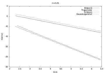
Figure 5: The logarithm of the error versus the logarithm of integration points for integral \( \frac{3}{2}\sqrt{x} \) computed by the Trapezoidal method and Simpson's rule (upper two lines), and Midpoint and Gauss-Legendre methods (lower two lines).

About object-oriented programming
From an implementational point of view, the advantage of class hierarchies in Python is that we can save coding by inheriting functionality from a superclass. In programming languages where each variable must be specified with a fixed type, class hierarchies are particularly useful because a function argument with a special type also works with all subclasses of that type. Suppose we have a function where we need to integrate:
def do_math(arg1, arg2, integrator):
    ...
    I = integrator.integrate(myfunc)
    ...
That is, integrator must be an instance of some class, or a
module, such that the syntax integrator.integrate(myfunc)
corresponds to a function call, but nothing more (like having a
particular type) is demanded.
This Python code will run as long as integrator has a method
integrate taking one argument. In other languages, the function
arguments are specified with a type, say in Java we would write
void do_math(double arg1, int arg2, Simpson integrator)
A compiler will examine all calls to do_math and control that the
arguments are of the right type. Instead of specifying the
integration method to be of type Simpson, one can in Java and other
object-oriented languages specify integrator to be of the superclass
type Integrator:
void do_math(double arg1, int arg2, Integrator integrator)
Now it is allowed to pass an object of any subclass type of
Integrator as the third argument. That is, this method works with
integrator of type Midpoint, Trapezoidal, Simpson, etc., not
just one of them. Class hierarchies and object-oriented programming
are therefore important means for parameterizing away types in
languages like Java, C++, and C#. We do not need to parameterize
types in Python, since arguments are not declared with a fixed
type. Object-oriented programming is hence not so technically
important in Python as in other languages for providing increased
flexibility in programs.
Is there then any use for object-oriented programming beyond
inheritance? The answer is yes! For many code developers
object-oriented programming is not just a technical way of sharing
code, but it is more a way of modeling the world, and understanding
the problem that the program is supposed to solve. In mathematical
applications we already have objects, defined by the mathematics, and
standard programming concepts such as functions, arrays, lists, and
loops are often sufficient for solving simpler problems. In the
non-mathematical world the concept of objects is very useful because
it helps to structure the problem to be solved. As an example, think
of the phone book and message list software in a mobile phone. Class
Person can be introduced to hold the data about one person in the
phone book, while class Message can hold data related to an SMS
message. Clearly, we need to know who sent a message so a Message
object will have an associated Person object, or just a phone number
if the number is not registered in the phone book. Classes help to
structure both the problem and the program. The impact of classes and
object-oriented programming on modern software development can hardly
be exaggerated.
A good, real-world, pedagogical example on inheritance is the class hierarchy for numerical methods for ordinary differential equations described in the document Programming of ordinary differential equations [4].