User interfaces

It is good programming practice to let programs read input from some user interface, rather than requiring users to edit parameter values in the source code. With effective user interfaces it becomes easier and safer to apply the code for scientific investigations and in particular to automate large-scale investigations by other programs (see the section Automating scientific experiments).

Reading input data can be done in many ways. We have to decide on the functionality of the user interface, i.e., how we want to operate the program when providing input. Thereafter, we use appropriate tools to implement that particular user interface. There are four basic types of user interface, listed here according to implementational complexity, from lowest to highest:

1. Questions and answers in the terminal window
2. Command-line arguments
3. Reading data from files
4. Graphical user interfaces (GUIs)

Personal preferences of user interfaces differ substantially, and it is difficult to present recommendations or pros and cons. Alternatives 2 and 4 are most popular and will be addressed next. The goal is to make it easy for the user to set physical and numerical parameters in our decay.py program. We use a little toy program, called prog.py, as introductory example:

delta = 0.5
p = 2
from math import exp
result = delta*exp(-p)
print result

The essential content is that prog.py has two input parameters: delta and p. A user interface will replace the first two assignments to delta and p.

Command-line arguments

The command-line arguments are all the words that appear on the command line after the program name. Running a program prog.py as python prog.py arg1 arg2 means that there are two command-line arguments (separated by white space): arg1 and arg2. Python stores all command-line arguments in a special list sys.argv. (The name argv stems from the C language and stands for “argument values”. In C there is also an integer variable called argc reflecting the number of arguments, or “argument counter”. A lot of programming languages have adopted the variable name argv for the command-line arguments.) Here is an example on a program what_is_sys_argv.py that can show us what the command-line arguments are

import sys
print sys.argv

A sample run goes like

Terminal> python what_is_sys_argv.py 5.0 'two words' -1E+4
['what_is_sys_argv.py', '5.0', 'two words', '-1E+4']

We make two observations:

• sys.argv[0] is the name of the program, and the sublist sys.argv[1:] contains all the command-line arguments.
• Each command-line argument is available as a string. A conversion to float is necessary if we want to compute with the numbers 5.0 and \(10^4\).

There are, in principle, two ways of programming with command-line arguments in Python:

• Positional arguments: Decide upon a sequence of parameters on the command line and read their values directly from the sys.argv[1:] list.
• Option-value pairs: Use --option value on the command line to replace the default value of an input parameter option by value (and utilize the argparse.ArgumentParser tool for implementation).

Suppose we want to run some program prog.py with specification of two parameters p and delta on the command line. With positional command-line arguments we write

Terminal> python prog.py 2 0.5

and must know that the first argument 2 represents p and the next 0.5 is the value of delta. With option-value pairs we can run

Terminal> python prog.py --delta 0.5 --p 2

Now, both p and delta are supposed to have default values in the program, so we need to specify only the parameter that is to be changed from its default value, e.g.,

Terminal> python prog.py --p 2         # p=2, default delta
Terminal> python prog.py --delta 0.7   # delta-0.7, default a
Terminal> python prog.py               # default a and delta

How do we extend the prog.py code for positional arguments and option-value pairs? Positional arguments require very simple code:

import sys
p = float(sys.argv[1])
delta = float(sys.argv[2])

from math import exp
result = delta*exp(-p)
print result

If the user forgets to supply two command-line arguments, Python will raise an IndexError exception and produce a long error message. To avoid that, we should use a try-except construction:

import sys
try:
    p = float(sys.argv[1])
    delta = float(sys.argv[2])
except IndexError:
    print 'Usage: %s p delta' % sys.argv[0]
    sys.exit(1)

from math import exp
result = delta*exp(-p)
print result

Using sys.exit(1) aborts the program. The value 1 (actually any value different from 0) notifies the operating system that the program failed.

Command-line arguments are strings

Note that all elements in sys.argv are string objects. If the values will enter mathematical computations, we need to explicitly convert the strings to numbers.

Option-value pairs requires more programming and is actually better explained in a more comprehensive example below. Minimal code for our prog.py program reads

import argparse
parser = argparse.ArgumentParser()
parser.add_argument('--p', default=1.0)
parser.add_argument('--delta', default=0.1)

args = parser.parse_args()
p = args.p
delta = args.delta

from math import exp
result = delta*exp(-p)
print result

Because the default values of delta and p are float numbers, the args.delta and args.p variable are automatically of type float.

Our next task is to use these basic code constructs to equip our decay.py module with command-line interfaces.

Positional command-line arguments

For our decay.py module file, we want include functionality such that we can read \(I\), \(a\), \(T\), \(\theta\), and a range of \(\Delta t\) values from the command line. A plot is then to be made, comparing the different numerical solutions for different \(\Delta t\) values against the exact solution. The technical details of getting the command-line information into the program is covered in the next two sections.

The simplest way of reading the input parameters is to decide on their sequence on the command line and just index the sys.argv list accordingly. Say the sequence of input data for some functionality in decay.py is \(I\), \(a\), \(T\), \(\theta\) followed by an arbitrary number of \(\Delta t\) values. This code extracts these positional command-line arguments:

def read_command_line_positional():
    if len(sys.argv) < 6:
        print 'Usage: %s I a T on/off BE/FE/CN dt1 dt2 dt3 ...' % \
              sys.argv[0]; sys.exit(1)  # abort

    I = float(sys.argv[1])
    a = float(sys.argv[2])
    T = float(sys.argv[3])
    theta = float(sys.argv[4])
    dt_values = [float(arg) for arg in sys.argv[5:]]

    return I, a, T, theta, dt_values

Note that we may use a try-except construction instead of the if test.

A run like

Terminal> python decay.py 1 0.5 4 0.5 1.5 0.75 0.1

results in

sys.argv = ['decay.py', '1', '0.5', '4', '0.5', '1.5', '0.75', '0.1']

and consequently the assignments I=1.0, a=0.5, T=4.0, thet=0.5, and dt_values = [1.5, 0.75, 0.1].

Instead of specifying the \(\theta\) value, we could be a bit more sophisticated and let the user write the name of the scheme: BE for Backward Euler, FE for Forward Euler, and CN for Crank-Nicolson. Then we must map this string to the proper \(\theta\) value, an operation elegantly done by a dictionary:

scheme = sys.argv[4]
scheme2theta = {'BE': 1, 'CN': 0.5, 'FE': 0}
if scheme in scheme2theta:
    theta = scheme2theta[scheme]
else:
    print 'Invalid scheme name:', scheme; sys.exit(1)

Now we can do

Terminal> python decay.py 1 0.5 4 CN 1.5 0.75 0.1

and get `theta=0.5`in the code.

Option-value pairs on the command line

Now we want to specify option-value pairs on the command line, using --I for I (\(I\)), --a for a (\(a\)), --T for T (\(T\)), --scheme for the scheme name (BE, FE, CN), and --dt for the sequence of dt (\(\Delta t\)) values. Each parameter must have a sensible default value so that we specify the option on the command line only when the default value is not suitable. Here is a typical run:

Terminal> python decay.py --I 2.5 --dt 0.1 0.2 0.01 --a 0.4

Observe the major advantage over positional command-line arguments: the input is much easier to read and much easier to write. With positional arguments it is easy to mess up the sequence of the input parameters and quite challenging to detect errors too, unless there are just a couple of arguments.

Python’s ArgumentParser tool in the argparse module makes it easy to create a professional command-line interface to any program. The documentation of ArgumentParser demonstrates its versatile applications, so we shall here just list an example containing the most basic features. It always pays off to use ArgumentParser rather than trying to manually inspect and interpret option-value pairs in sys.argv!

The use of ArgumentParser typically involves three steps:

import argparse
parser = argparse.ArgumentParser()

# Step 1: add arguments
parser.add_argument('--option_name', ...)

# Step 2: interpret the command line
args = parser.parse_args()

# Step 3: extract values
value = args.option_name

A function for setting up all the options is handy:

def define_command_line_options():
    import argparse
    parser = argparse.ArgumentParser()
    parser.add_argument(
        '--I', '--initial_condition', type=float,
        default=1.0, help='initial condition, u(0)',
        metavar='I')
    parser.add_argument(
        '--a', type=float, default=1.0,
        help='coefficient in ODE', metavar='a')
    parser.add_argument(
        '--T', '--stop_time', type=float,
        default=1.0, help='end time of simulation',
        metavar='T')
    parser.add_argument(
        '--scheme', type=str, default='CN',
        help='FE, BE, or CN')
    parser.add_argument(
        '--dt', '--time_step_values', type=float,
        default=[1.0], help='time step values',
        metavar='dt', nargs='+', dest='dt_values')
    return parser

Each command-line option is defined through the parser.add_argument method [1]. Alternative options, like the short --I and the more explaining version --initial_condition can be defined. Other arguments are type for the Python object type, a default value, and a help string, which gets printed if the command-line argument -h or --help is included. The metavar argument specifies the value associated with the option when the help string is printed. For example, the option for \(I\) has this help output:

Terminal> python decay.py -h
  ...
  --I I, --initial_condition I
                        initial condition, u(0)
  ...

The structure of this output is

--I metavar, --initial_condition metavar
                      help-string

[1]	We use the expression method here, because parser is a class variable and functions in classes are known as methods in Python and many other languages. Readers not familiar with class programming can just substitute this use of method by function.

Finally, the --dt option demonstrates how to allow for more than one value (separated by blanks) through the nargs='+' keyword argument. After the command line is parsed, we get an object where the values of the options are stored as attributes. The attribute name is specified by the dist keyword argument, which for the --dt option is dt_values. Without the dest argument, the value of an option --opt is stored as the attribute opt.

The code below demonstrates how to read the command line and extract the values for each option:

def read_command_line_argparse():
    parser = define_command_line_options()
    args = parser.parse_args()
    scheme2theta = {'BE': 1, 'CN': 0.5, 'FE': 0}
    data = (args.I, args.a, args.T, scheme2theta[args.scheme],
            args.dt_values)
    return data

As seen, the values of the command-line options are available as attributes in args: args.opt holds the value of option --opt, unless we used the dest argument (as for --dt_values) for specifying the attribute name. The args.opt attribute has the object type specified by type (str by default).

The making of the plot is not dependent on whether we read data from the command line as positional arguments or option-value pairs:

def experiment_compare_dt(option_value_pairs=False):
    I, a, T, theta, dt_values = \
       read_command_line_argparse() if option_value_pairs else \
       read_command_line_positional()

    legends = []
    for dt in dt_values:
        u, t = solver(I, a, T, dt, theta)
        plt.plot(t, u)
        legends.append('dt=%g' % dt)
    t_e = np.linspace(0, T, 1001)       # very fine mesh for u_e
    u_e = exact_solution(t_e, I, a)
    plt.plot(t_e, u_e, '--')
    legends.append('exact')
    plt.legend(legends, loc='upper right')
    plt.title('theta=%g' % theta)
    plotfile = 'tmp'
    plt.savefig(plotfile + '.png');  plt.savefig(plotfile + '.pdf')

Creating a graphical web user interface

The Python package Parampool can be used to automatically generate a web-based graphical user interface (GUI) for our simulation program. Although the programming technique dramatically simplifies the efforts to create a GUI, the forthcoming material on equipping our decay module with a GUI is quite technical and of significantly less importance than knowing how to make a command-line interface.

Making a compute function

The first step is to identify a function that performs the computations and that takes the necessary input variables as arguments. This is called the compute function in Parampool terminology. The purpose of this function is to take values of \(I\), \(a\), \(T\) together with a sequence of \(\Delta t\) values and a sequence of \(\theta\) and plot the numerical against the exact solution for each pair of \((\theta, \Delta t)\). The plots can be arranged as a table with the columns being scheme type (\(\theta\) value) and the rows reflecting the discretization parameter (\(\Delta t\) value). Figure Automatically generated graphical web interface displays what the graphical web interface may look like after results are computed (there are \(3\times 3\) plots in the GUI, but only \(2\times 2\) are visible in the figure).

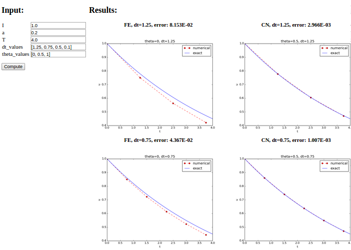
Automatically generated graphical web interface

To tell Parampool what type of input data we have, we assign default values of the right type to all arguments in the compute function, here called main_GUI:

def main_GUI(I=1.0, a=.2, T=4.0,
             dt_values=[1.25, 0.75, 0.5, 0.1],
             theta_values=[0, 0.5, 1]):

The compute function must return the HTML code we want for displaying the result in a web page. Here we want to show a table of plots. Assume for now that the HTML code for one plot and the value of the norm of the error can be computed by some other function compute4web. The main_GUI function can then loop over \(\Delta t\) and \(\theta\) values and put each plot in an HTML table. Appropriate code goes like

def main_GUI(I=1.0, a=.2, T=4.0,
             dt_values=[1.25, 0.75, 0.5, 0.1],
             theta_values=[0, 0.5, 1]):
    # Build HTML code for web page. Arrange plots in columns
    # corresponding to the theta values, with dt down the rows
    theta2name = {0: 'FE', 1: 'BE', 0.5: 'CN'}
    html_text = '<table>\n'
    for dt in dt_values:
        html_text += '<tr>\n'
        for theta in theta_values:
            E, html = compute4web(I, a, T, dt, theta)
            html_text += """
<td>
<center><b>%s, dt=%g, error: %.3E</b></center><br>
%s
</td>
""" % (theta2name[theta], dt, E, html)
        html_text += '</tr>\n'
    html_text += '</table>\n'
    return html_text

Making one plot is done in compute4web. The statements should be straightforward from earlier examples, but there is one new feature: we use a tool in Parampool to embed the PNG code for a plot file directly in an HTML image tag. The details are hidden from the programmer, who can just rely on relevant HTML code in the string html_text. The function looks like

def compute4web(I, a, T, dt, theta=0.5):
    """
    Run a case with the solver, compute error measure,
    and plot the numerical and exact solutions in a PNG
    plot whose data are embedded in an HTML image tag.
    """
    u, t = solver(I, a, T, dt, theta)
    u_e = exact_solution(t, I, a)
    e = u_e - u
    E = np.sqrt(dt*np.sum(e**2))

    plt.figure()
    t_e = np.linspace(0, T, 1001)    # fine mesh for u_e
    u_e = exact_solution(t_e, I, a)
    plt.plot(t,   u,   'r--o')
    plt.plot(t_e, u_e, 'b-')
    plt.legend(['numerical', 'exact'])
    plt.xlabel('t')
    plt.ylabel('u')
    plt.title('theta=%g, dt=%g' % (theta, dt))
    # Save plot to HTML img tag with PNG code as embedded data
    from parampool.utils import save_png_to_str
    html_text = save_png_to_str(plt, plotwidth=400)

    return E, html_text

Generating the user interface

The web GUI is automatically generated by the following code, placed in the file decay_GUI_generate.py.

from parampool.generator.flask import generate
from decay import main_GUI
generate(main_GUI,
         filename_controller='decay_GUI_controller.py',
         filename_template='decay_GUI_view.py',
         filename_model='decay_GUI_model.py')

Running the decay_GUI_generate.py program results in three new files whose names are specified in the call to generate:

1. decay_GUI_model.py defines HTML widgets to be used to set input data in the web interface,
2. templates/decay_GUI_views.py defines the layout of the web page,
3. decay_GUI_controller.py runs the web application.

We only need to run the last program, and there is no need to look into these files.

Running the web application

The web GUI is started by

Terminal> python decay_GUI_controller.py

Open a web browser at the location 127.0.0.1:5000. Input fields for I, a, T, dt_values, and theta_values are presented. Figure Automatically generated graphical web interface shows a part of the resulting page if we run with the default values for the input parameters. With the techniques demonstrated here, one can easily create a tailored web GUI for a particular type of application and use it to interactively explore physical and numerical effects.