Basic implementations

Mathematical problem and solution technique

We address the perhaps simplest possible differential equation problem

(1)\[ u'(t) = -au(t), \quad t \in (0,T],\]

(2)\[ u(0) = I,\]

where \(a\), \(I\), and \(T\) are prescribed parameters, and \(u(t)\) is the unknown function to be estimated. This mathematical model is relevant for physical phenomena featuring exponential decay in time, e.g., vertical pressure variation in the atmosphere, cooling of an object, and radioactive decay.

The time domain is discretized with points \(0 = t_0 < t_1 \cdots < t_{N_t}=T\), here with a constant spacing \(\Delta t\) between the mesh points: \(\Delta t = t_{n}-t_{n-1}\), \(n=1,\ldots,N_t\). Let \(u^n\) be the numerical approximation to the exact solution at \(t_n\). A family of popular numerical methods can be written in the form

(3)\[ u^{n+1} = \frac{1 - (1-\theta) a\Delta t}{1 + \theta a\Delta t}u^n,\]

for \(n=0,1,\ldots,N_t-1\). This numerical scheme corresponds to the Forward Euler scheme when \(\theta=0\), the Backward Euler scheme when \(\theta=1\), and the Crank-Nicolson scheme when \(\theta=1/2\). The initial condition (2) is key to start the recursion with a value for \(u^0\).

A first, quick implementation

Solving (3) in a program is very straightforward: just make a loop over \(n\) and evaluate the formula. The \(u(t_n\)) values for discrete \(n\) can be stored in an array. This makes it easy to also plot the solution. It would be natural to also add the exact solution curve \(u(t)=Ie^{-at}\) to the plot.

We apply the Python programming language since it gives code close to that of other popular languages such as MATLAB and R. The programming habits of many students and engineers would lead them to write a program like this:

from numpy import *
from matplotlib.pyplot import *

A = 1
a = 2
T = 4
dt = 0.2
N = int(round(T/dt))
y = zeros(N+1)
t = linspace(0, T, N+1)
theta = 1
y[0] = A
for n in range(0, N):
    y[n+1] = (1 - (1-theta)*a*dt)/(1 + theta*dt*a)*y[n]

y_e = A*exp(-a*t) - y
error = y_e - y
E = sqrt(dt*sum(error**2))
print 'Norm of the error: %.3E' % E
plot(t, y, 'r--o')
t_e = linspace(0, T, 1001)
y_e = A*exp(-a*t_e)
plot(t_e, y_e, 'b-')
legend(['numerical, theta=%g' % theta, 'exact'])
xlabel('t')
ylabel('y')
show()

This program is easy to read, and as long it is correct, many will claim that it has sufficient quality. Nevertheless, the program suffers from two serious flaws:

1. The notation in the program does not correspond exactly to the notation in the mathematical problem: the solution is called y and corresponds to \(u\) in the mathematical description, the variable A corresponds to the mathematical parameter \(I\), N in the program is called \(N_t\) in the mathematics.
2. There are no comments in the program.

These kind of flaws quickly become crucial if present in code for complicated mathematical problems and code that is meant to be extended to other problems.

We also note that the program is “flat” in the sense that it does not contain functions. Usually, this is a bad habit, but let us correct the two mentioned flaws first.

A more decent program

A code of better quality arises from fixing the notation and adding comments:

from numpy import *
from matplotlib.pyplot import *

I = 1
a = 2
T = 4
dt = 0.2
Nt = int(round(T/dt))     # no of time intervals
u = zeros(Nt+1)           # array of u[n] values
t = linspace(0, T, Nt+1)  # time mesh
theta = 1                 # Backward Euler method

u[0] = I                  # assign initial condition
for n in range(0, Nt):    # n=0,1,...,Nt-1
    u[n+1] = (1 - (1-theta)*a*dt)/(1 + theta*dt*a)*u[n]

# Compute norm of the error
u_e = I*exp(-a*t) - u     # exact u at the mesh points
error = u_e - u
E = sqrt(dt*sum(error**2))
print 'Norm of the error: %.3E' % E

# Compare numerical (u) and exact solution (u_e) in a plot
plot(t, u, 'r--o')
t_e = linspace(0, T, 1001)       # very fine mesh for u_e
u_e = I*exp(-a*t_e)
plot(t_e, u_e, 'b-')
legend(['numerical, theta=%g' % theta, 'exact'])
xlabel('t')
ylabel('u')
show()

Comments

There is obviously not just one way to comment a program, and opinions may differ as to what code should be accomplished by comments. The guiding principle is, however, that comments should make the program easy to understand for human eye. Do not comment obvious constructions, but focus on ideas and (“what happens in the next statements?”) and on explaining code that can be interpreted as complicated.

Refactoring into functions

At first sight, our updated program seems like a good starting point for playing around with the mathematical problem: we can just change parameters and rerun. Although such edit-and-rerun sessions are good for initial exploration, one will soon extend the experiments and start developing the code further. Say we want to compare \(\theta =0,1,0.5\) in the same plot. This extension requires changes all over the code and quickly leads to errors. To do something serious with this program, we have to break it into smaller pieces and make sure each piece is well tested, and ensure that the program is sufficiently general and can be reused in new contexts without changes. The next natural step is therefore to isolate the numerical computations and the visualization in separate Python functions. Such a rewrite of a code, without essentially changing the functionality, but just improve the quality of the code, is known as refactoring. After one has quickly put some code down and tested it, it is a common step to refactor it so it is better prepared for extensions.

Program file vs IDE vs notebook

There are basically three different ways of working with Python code:

1. One writes the code in a file, using a text editor (such as Emacs or Vim) and runs it in a terminal window.
2. One applies an Integrated Development Environment (the simplest is IDLE, which comes with standard Python) containing a graphical user interface with an editor and an element where Python code can be run.
3. One applies the Jupyter Notebook (previously known as IPython Notebook), which offers an interactive environment for Python code where plots are automatically inserted after the code, see Figure Experimental code in a notebook.

It appears that method 1 and 2 are quite equivalent, but the notebook encourages more experimental code in flat programs. Therefore, notebook users will normally need to think more about refactoring code and increase the use of functions.

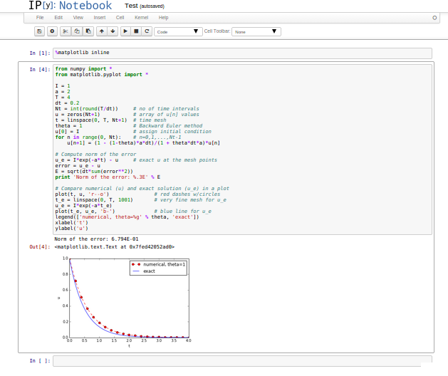
Experimental code in a notebook

Implementing the numerical algorithm in a function

The solution formula (3) is completely general and should be available as a Python function solver with all input data as function arguments and all output data returned to the calling code. With this solver function we can solve all types of problems (1)-(2) by an easy-to-read one-line statement:

u, t = solver(I=1, a=2, T=4, dt=0.2, theta=0.5)

Refactoring the numerical method in the previous flat program in terms of a solver function leads to this code:

def solver(I, a, T, dt, theta):
    """Solve u'=-a*u, u(0)=I, for t in (0,T] with steps of dt."""
    dt = float(dt)               # avoid integer division
    Nt = int(round(T/dt))        # no of time intervals
    T = Nt*dt                    # adjust T to fit time step dt
    u = np.zeros(Nt+1)           # array of u[n] values
    t = np.linspace(0, T, Nt+1)  # time mesh

    u[0] = I                  # assign initial condition
    for n in range(0, Nt):    # n=0,1,...,Nt-1
        u[n+1] = (1 - (1-theta)*a*dt)/(1 + theta*dt*a)*u[n]
    return u, t

Tip: Always use a doc string to document a function

Python has a convention for documenting the purpose and usage of a function in a doc string: simply place the documentation in a one- or multi-line triple-quoted string right after the function header.

Be careful with unintended integer division

Note that we in the solver function explicitly covert dt to a float object. If not, the updating formula for u[n+1] may evaluate to zero because of integer division when theta, a, and dt are integers!

Do not have several versions of a code

One of the most serious flaws in computational work is to have several slightly different implementations of the same computational algorithms lying around in various program files. This is very likely to happen, because busy scientists often want to test a slight variation of a code to see what happens. A quick copy-and-edit does the task, but such quick hacks tend to survive. When a real correction is needed in the implementation, it is difficult to ensure that the correction is done in all relevant files. In fact, this is a general problem in programming, which has led to an important principle.

The DRY principle: Don’t repeat yourself

When implementing a particular functionality in a computer program, make sure this functionality and its variations are implemented in just one piece of code. That is, if you need to revise the implementation, there should be one and only one place to edit. It follows that you should never duplicate code (don’t repeat yourself!), and code snippets that are similar should be factored into one piece (function) and parameterized (by function arguments).

The DRY principle means that our solver function should not be copied to a new file if we need some modifications. Instead, we should try to extend solver such that the new and old needs are met by a single function. Sometimes this process requires a new refactoring, but having a numerical method in one and only one place is a great advantage.

Making a module

As soon as you start making Python functions in a program, you should make sure the program file fulfills the requirement of a module. This means that you can import and reuse your functions in other programs too. For example, if our solver function resides in a module file decay.py, another program may reuse of the function either by

from decay import solver
u, t = solver(I=1, a=2, T=4, dt=0.2, theta=0.5)

or by a slightly different import statement, combined with a subsequent prefix of the function name by the name of the module:

import decay
u, t = decay.solver(I=1, a=2, T=4, dt=0.2, theta=0.5)

The requirements for a program file to also qualify for a module are simple:

1. The filename without .py must be a valid Python variable name.
2. The main program must be executed (through statements or a function call) in the test block.

The test block is normally placed at the end of a module file:

if __name__ == '__main__':
    # Statements

When the module file is executed as a stand-alone program, the if test is true and the indented statements are run. If the module file is imported, however, __name__ equals the module name and the test block is not executed.

To demonstrate the difference, consider the trivial module file hello.py with one function and a call to this function as main program:

def hello(arg='World!'):
    print 'Hello, ' + arg

if __name__ == '__main__':
    hello()

Without the test block, the code reads

def hello(arg='World!'):
    print 'Hello, ' + arg

hello()

With this latter version of the file, any attempt to import hello will, at the same time, execute the call hello() and hence write “Hello, World!” to the screen. Such output is not desired when importing a module! To make import and execution of code independent for another program that wants to use the function hello, the module hello must be written with a test block. Furthermore, running the file itself as python hello.py will make the block active and lead to the desired printing.

All coming functions are placed in a module

The many functions to be explained in the following text are put in one module file decay.py.

What more than the solver function is needed in our decay module to do everything we did in the previous, flat program? We need import statements for numpy and matplotlib as well as another function for producing the plot. It can also be convenient to put the exact solution in a Python function. Our module decay.py then looks like this:

from numpy import *
from matplotlib.pyplot import *

def solver(I, a, T, dt, theta):
    ...

def exact_solution(t, I, a):
    return I*exp(-a*t)

def experiment_compare_numerical_and_exact():
    I = 1;  a = 2;  T = 4;  dt = 0.4;  theta = 1
    u, t = solver(I, a, T, dt, theta)

    t_e = linspace(0, T, 1001)       # very fine mesh for u_e
    u_e = exact_solution(t_e, I, a)

    plot(t,   u,   'r--o')           # dashed red line with circles
    plot(t_e, u_e, 'b-')             # blue line for u_e
    legend(['numerical, theta=%g' % theta, 'exact'])
    xlabel('t')
    ylabel('u')
    plotfile = 'tmp'
    savefig(plotfile + '.png');  savefig(plotfile + '.pdf')

    error = exact_solution(t, I, a) - u
    E = sqrt(dt*sum(error**2))
    print 'Error norm:', E

if __name__ == '__main__':
    experiment_compare_numerical_and_exact()

This module file does exactly the same as the previous, flat program, but now it becomes much easier to extend the code with more functions that produce other plots, other experiments, etc. Even more important, though, is that the numerical algorithm is coded and tested once and for all in the solver function, and any need to solve the mathematical problem is a matter of one function call.

Prefixing imported functions by the module name

Import statements of the form from module import * import all functions and variables in module.py into the current file. This is often referred to as “import star”, and many find this convenient, but it is not considered as a good programming style in Python. For example, when doing

from numpy import *
from matplotlib.pyplot import *

we get mathematical functions like sin and exp as well as MATLAB-style functions like linspace and plot, which can be called by these well-known names. Unfortunately, it sometimes becomes confusing to know where a particular function comes from, i.e., what modules you need to import. Is a desired function from numpy or matplotlib.pyplot? Or is it our own function? These questions are easy to answer if functions in modules are prefixed by the module name. Doing an additional from math import * is really crucial: now sin, cos, and other mathematical functions are imported and their names hide those previously imported from numpy. That is, sin is now a sine function that accepts a float argument, not an array.

Doing the import such that module functions must have a prefix is generally recommended:

import numpy
import matplotlib.pyplot

t = numpy.linspace(0, T, Nt+1)
u_e = I*numpy.exp(-a*t)
matplotlib.pyplot.plot(t, u_e)

The modules numpy and matplotlib.pyplot are frequently used, and since their full names are quite tedious to write, two standard abbreviations have evolved in the Python scientific computing community:

import numpy as np
import matplotlib.pyplot as plt

t = np.linspace(0, T, Nt+1)
u_e = I*np.exp(-a*t)
plt.plot(t, u_e)

The downside of prefixing functions by the module name is that mathematical expressions like \(e^{-at}\sin(2\pi t)\) get cluttered with module names,

numpy.exp(-a*t)*numpy.sin(2(numpy.pi*t)
# or
np.exp(-a*t)*np.sin(2*np.pi*t)

Such an expression looks like exp(-a*t)*sin(2*pi*t) in most other programming languages. Similarly, np.linspace and plt.plot look less familiar to people who are used to MATLAB and who have not adopted Python’s prefix style. Whether to do from module import * or import module depends on personal taste and the problem at hand. In these writings we use from module import in more basic, shorter programs where similarity with MATLAB could be an advantage. Prefix of mathematical functions in formulas is something we often avoid to obtain a one-to-one correspondence between mathematical formulas and the Python code.

Our decay module can be edited to use the module prefix for matplotlib.pyplot and numpy:

import numpy as np
import matplotlib.pyplot as plt

def solver(I, a, T, dt, theta):
    ...

def exact_solution(t, I, a):
    return I*np.exp(-a*t)

def experiment_compare_numerical_and_exact():
    I = 1;  a = 2;  T = 4;  dt = 0.4;  theta = 1
    u, t = solver(I, a, T, dt, theta)

    t_e = np.linspace(0, T, 1001)       # very fine mesh for u_e
    u_e = exact_solution(t_e, I, a)

    plt.plot(t,   u,   'r--o')       # dashed red line with circles
    plt.plot(t_e, u_e, 'b-')         # blue line for u_e
    plt.legend(['numerical, theta=%g' % theta, 'exact'])
    plt.xlabel('t')
    plt.ylabel('u')
    plotfile = 'tmp'
    plt.savefig(plotfile + '.png');  plt.savefig(plotfile + '.pdf')

    error = exact_solution(t, I, a) - u
    E = np.sqrt(dt*np.sum(error**2))
    print 'Error norm:', E

if __name__ == '__main__':
    experiment_compare_numerical_and_exact()

Without the prefix, the import and mathematical formulas read

from numpy import exp, sum, sqrt

def exact_solution(t, I, a):
    return I*exp(-a*t)

error = exact_solution(t, I, a) - u
E = sqrt(dt*sum(error**2))

Example on extending the module code

Let us specifically demonstrate one extension of the flat program in the section A first, quick implementation that would require substantial editing of the flat code (the section A more decent program), while in a structured module (the section Making a module), we can simply add a new function without affecting the existing code.

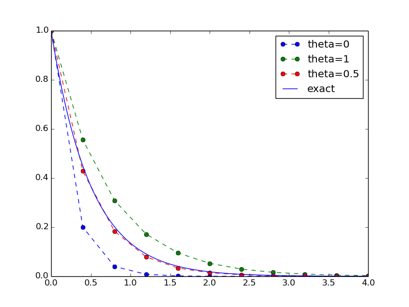
Our example that illustrates the extension is to make a comparison between the numerical solutions for various schemes (\(\theta\) values) and the exact solution:

Wait a minute

Look at the flat program in the section A first, quick implementation, and try to imagine which edits that are required to solve this new problem.

With the solver function at hand, we can simply create a function with a loop over theta values and add the necessary plot statements:

def experiment_compare_schemes():
    """Compare theta=0,1,0.5 in the same plot."""
    I = 1;  a = 2;  T = 4;  dt = 0.4
    legends = []
    for theta in [0, 1, 0.5]:
        u, t = solver(I, a, T, dt, theta)
        plt.plot(t, u, '--o')
        legends.append('theta=%g' % theta)
    t_e = np.linspace(0, T, 1001)        # very fine mesh for u_e
    u_e = exact_solution(t_e, I, a)
    plt.plot(t_e, u_e, 'b-')
    legends.append('exact')
    plt.legend(legends, loc='upper right')
    plotfile = 'tmp'
    plt.savefig(plotfile + '.png');  plt.savefig(plotfile + '.pdf')

A call to this experiment_compare_schemes function must be placed in the test block, or you can run the program from IPython instead:

In[1]: from decay import *

In[2]: experiment_compare_schemes()

We do not present how the flat program from the section A more decent program must be refactored to produce the desired plots, but simply state that the danger of introducing bugs is significantly larger than when just writing an additional function in the decay module.

Documenting functions and modules

We have already emphasized the importance of documenting functions with a doc string (see the section Implementing the numerical algorithm in a function). Now it is time to show how doc strings should be structured in order to take advantage of the documentation utilities in the numpy module. The idea is to follow a convention that in itself makes a good pure text doc string in the terminal window and at the same time can be translated to beautiful HTML manuals for the web.

The conventions for numpy style doc strings are well documented, so here we just present a basic example that the reader can adopt. Input arguments to a function are listed under the heading Parameters, while returned values are listed under Returns. It is a good idea to also add an Examples section on the usage of the function. More complicated software may have additional sections, see pydoc numpy.load for an example. The markup language available for doc strings is Sphinx-extended reStructuredText. The example below shows typical constructs: 1) how inline mathematics is written with the :math: directive, 2) how arguments to the functions are referred to using single backticks (inline monospace font for code applies double backticks), and 3) how arguments and return values are listed with types and explanation.

def solver(I, a, T, dt, theta):
    """
    Solve  \( u'=-au \)  with  \( u(0)=I \)  for  \( t \in (0,T] \) 
    with steps of `dt` and the method implied by `theta`.

    Parameters
    ----------
    I: float
        Initial condition.
    a: float
        Parameter in the differential equation.
    T: float
        Total simulation time.
    theta: float, int
        Parameter in the numerical scheme. 0 gives
        Forward Euler, 1 Backward Euler, and 0.5
        the centered Crank-Nicolson scheme.

    Returns
    -------
    `u`: array
        Solution array.
    `t`: array
        Array with time points corresponding to `u`.

    Examples
    --------
    Solve  \( u' = -\\frac{1}{2}u, u(0)=1.5 \) 
    with the Crank-Nicolson method:

    >>> u, t = solver(I=1.5, a=0.5, T=9, theta=0.5)
    >>> import matplotlib.pyplot as plt
    >>> plt.plot(t, u)
    >>> plt.show()
    """

If you follow such doc string conventions in your software, you can easily produce nice manuals that meet the standard expected within the Python scientific computing community.

Sphinx requires quite a number of manual steps to prepare a manual, so it is recommended to use a premade script to automate the steps. (You need to do a pip install of sphinx and numpydoc to make the script work.) Figure Example on Sphinx API manual in HTML provides an example of what the above doc strings look like when Sphinx has transformed them to HTML.

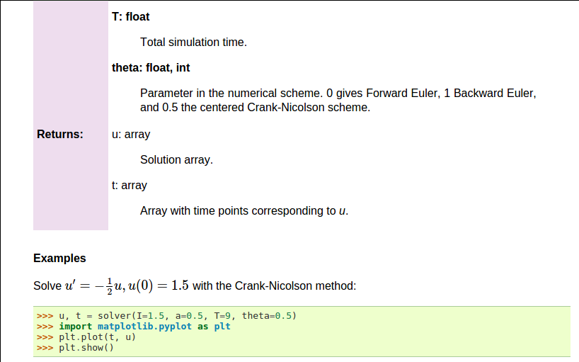
Example on Sphinx API manual in HTML