FEniCS solver with optimization in Octave

While Python has gained significant momentum in scientific computing in recent years, Matlab and its open source counterpart Octave are still much more dominating tools in the community. There are tons of MATLAB/Octave code around that FEniCS users may like to take advantage of. Fortunately, MATLAB and Octave both have Python interfaces so it is straightforward to call MATLAB/Octave from FEniCS simulators implemented in Python. The technical details of such coupling is the presented with the aid of an example.

Basic use of Pytave

First we show how to operate Octave from Python. Our focus is on the Octave interface named Pytave. The basic Pytave command is

result = pytave.feval(n, "func", A, B, ...)

for running the function func in the Octave engine with arguments A, B, and so forth, resulting in n returned objects to Python. For example, computing the eigenvalues of a matrix is done by

import numpy, pytave
A = numpy.random.random([2,2])
e = pytave.feval(1, "eig", A)
print 'Eigenvalues:', e

The eigenvalues and eigenvectors of a generalized eigenvalue problem \(A v = \lambda B v\) is computed by obtain both the eigenvalues and the eigenvectors, we do

A = numpy.random.random([2,2])
B = numpy.random.random([2,2])
e, v = pytave.feval(2, "eig", A, B)
print 'Eigenvalues:', e
print 'Eigenvectors:', v

Note that we here have two input arguments, A and B, and two output arguments, e and v (and because of the latter the first argument to feval is 2).

We could equally well solved these eigenvalue problems directly in numpy without any need for Octave, but the next example shows how to take advantage of a package with many MATLAB/Octave files offering functionality that is not available in Python.

Calling the MATLAB/Octave software

The following scientific application involves the coupling of our FEniCS flow solver with a MATLAB/Octave toolbox for solving optimization problems based on Kriging and the surrogate managment method. Our task is to minimize the fluid velocity in a certain region by placing a porous media within the domain. We can choose the size, placement and permeability of the porous media, but are not allowed to affect the pressure drop from the inlet to the outlet much. Figures Velocity problem around a porous media with and Velocity problem around a porous media with near optimal values: show the flow velocity with two different placements of two different porous media.

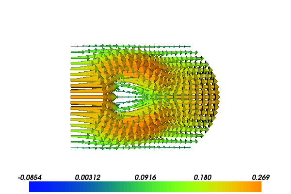
Velocity problem around a porous media with \(K_0=1000, x_0 = 0.4, c=0.1\)

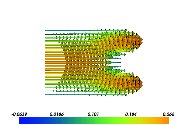
Velocity problem around a porous media with near optimal values: \(K_0=564, x_0 = 0.92, c=0.10\)

For this particular application we assume that the Reynolds number is low such that the flow can be modeled by the Stokes problem. Furthermore, the additional resistance caused by the porous medium is modeled by a positive lower order term \(K u\) resulting in the Brinkman model. The equations then reads

\[-\Delta u + K u - \nabla p = 0,\quad \mbox{ in }\Omega\]

\[\nabla \cdot u = 0,\quad \mbox{ in } \Omega\]

\[ u = (0,0),\quad \mbox{ on } y=0,1\]

\[u = (y(1-y),0),\quad \mbox{ on } x=0\]

\[\frac{\partial u}{\partial n} + p n = 0,\quad \mbox{ on } x=1\]

with

\[K = K_0 \mbox{ if } |x - x_0 | \leq c,\ | y - 0.5 | \leq c,\]

while \(K=0\) outside this rectangular region.

When \(K=0\) we have viscous Stokes flow while inside the porous medium, \(K=K_0\), and the \(K u\) term in the equation dominates over the viscous term \(\Delta u\).

The goal functional that we seek to minimize is

\[J(K_0, x_0, c) = u_x|_{(x=1,y=0.5)} + \int_\Omega (\nabla p)^2 \, dx\]

Here, \(u\) and \(p\) are functions of \(K_0\), \(x_0\), and \(c\), and \(u_x\) is the \(x\) component of \(u\).

The MATLAB/Octave code for the surrogate management and Kriging is based on Dace, but has been extended by Alison Marsden et. al. cite{Marsden_et_al_2004, Marsden_et_al_2008, Marsden_et_al_2012} to implement surrogate management. This algorithm consists of four main steps 1) search, 2) poll, 3) refine and 4) run simulations, with a flow chart appearing in Figure The flow chart of the surrogate management method. The two first steps find new sample points \(K_0\), \(x_0\), and \(c\), while refine increases the resolution in the parameter space, and finally the fourth step runs simulations with the new sample points.

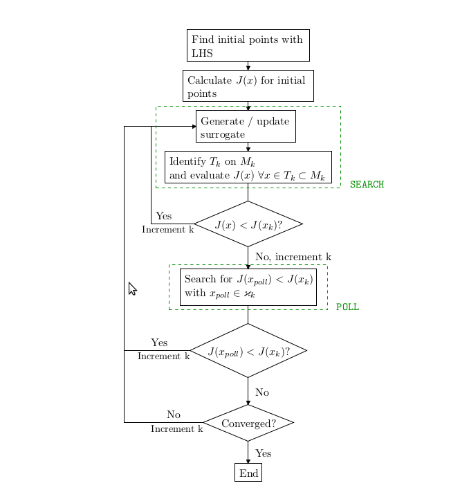
The flow chart of the surrogate management method

The main algorithm is implemented in Python (file opimize_flow_by_SMF.py) and listed below. It calls three key Python functions: search, poll, and refine, which make calls to the MATLAB/Octave package.

# main loop
while nit <= max_nit and refine_ok and not converged:
   # search step
   if cost_improve:
       Ai_new = search(Aall, Jall, curr_bestA, theta,
                       upb, lob, N, amin, amax, spc, delta)
       prev_it = "search"
       Ai_new = coarsen(Ai_new)
   else:
       # poll step
       if prev_it == "search":
           Ai_new = poll(Aall, Jall, curr_bestA, N,
                         delta, spc, amin, amax)
           prev_it = "poll"
       # refine if previous poll did not lead to cost improvement
       if prev_it == "poll":
           refine_ok, delta, spc = refine(delta, deltamin, spc)
           if refine_ok:
               Ai_new = search(Aall, Jall, curr_bestA, theta,
                               upb, lob, N, amin, amax, spc, delta)
               prev_it = "search"
           else:
               Ai_new = None
   nit += 1

   # run simulations on the new parameters
   if not Ai_new == None:
       Ai_new, J_new = run_simulations(Ai_new)

       # stack the new runs to the previous
       Jall = numpy.hstack((Jall, J_new))
       Aall = numpy.vstack((Aall, Ai_new))

       # monitor convergence (write to files)
       monitor(Aall, Jall, nit, curr_bestA, curr_bestJ,
               delta, prev_it, improve, spc)

       # check convergence
       cost_improve, curr_bestA, curr_bestJ = check(
           Ai_new, J_new, nit, curr_bestJ, curr_bestA)
   else:
       cost_improve = 0

The search and poll steps are both implemented in Python but are mainly wrappers around MATLAB/Octave functions. The search step is implemented as follows:

def search(Aall, Jall, curr_bestA, theta, upb,
           lob, N, amin, amax, spc, delta):
    """Search step."""
     # make sure that all points are unique
    (Am, Jm) = pytave.feval(2, "dsmerge", Aall, Jall)

    next_ptsall = []
    next_pts = None
    max_no_searches = 100
    no_searches = 0
    while next_pts == None and no_searches < max_no_searches:
        next_ptsall, min_est, max_mse_pt = pytave.feval(
            3, "krig_min_find_MADS_oct",
            Am, Jm, curr_bestA, theta, upb, lob,
            N, amin, amax, spc, delta)
        next_pts = check_for_new_points(next_ptsall, Aall)
        no_searches += 1
    return next_pts

Here, dsmerge and krig_min_find_MADS_oct are functions available in the MATLAB/Octave files dsmerge.m and krig_min_find_MADS_oct.m. We need to notify Octave about the directory (SMF) where these files can be found:

pytave.feval(0, "addpath", "SMF")

The FEniCS PDE solver

The FEniCS solver first defines the inflow condition (class EssentialBC), the K coefficient in the PDEs, and the Dirichlet boundary:

class EssentialBC(Expression):
    def eval(self, v, x):
        if x[0] < DOLFIN_EPS:
            y = x[1]
            v[0] = y*(1-y);  v[1] = 0
        else:
            v[0] = 0; v[1] = 0

    def value_shape(self):
        return (2,)

class K(Expression):
    def __init__(self, K0, x0, c):
        self.K0, self.x0, self.c = K0, x0, c

    def eval(self, v, x):
        x0, K0, c = self.x0, self.K0, self.c
        if abs(x[0] - x0) <= c and abs(x[1] - 0.5) <= c:
            v[0] = K0
        else:
            v[0] = 1

def dirichlet_boundary(x):
    return bool(x[0] < DOLFIN_EPS or x[1] < DOLFIN_EPS or \
                x[1] > 1.0 - DOLFIN_EPS)

The core of the solver is the following class:

class FlowProblem2Optimize:
    def __init__(self, K0, x0, c, plot):
        self.K0, self.x0, self.c, self.plot = K0, x0, c, plot

    def run(self):
        K0, x0, c = self.K0, self.x0, self.c

        mesh = UnitSquareMesh(20, 20)
        V = VectorFunctionSpace(mesh, "Lagrange", 2)
        Q = FunctionSpace(mesh, "Lagrange", 1)
        W = MixedFunctionSpace([V,Q])
        u, p = TrialFunctions(W)
        v, q = TestFunctions(W)
        k = K(K0, x0, c)

        u_inflow = EssentialBC()
        bc = DirichletBC(W.sub(0), u_inflow, dirichlet_boundary)
        f = Constant(0)

        a = inner(grad(u), grad(v))*dx + k*inner(u, v)*dx + \
            div(u)*q*dx + div(v)*p*dx
        L = f*q*dx

        w = Function(W)
        solve(a == L, w, bc)

        u, p = w.split()
        u1, u2 = split(u)

        goal1 = assemble(inner(grad(p), grad(p))*dx)
        goal2 = u(1.0, 0.5)[0]*1000
        goal = goal1 + goal2

        if self.plot:
            plot(u)

        key_variables = dict(K0=K0, x0=x0, c=c, goal1=goal1,
                             goal2=goal2, goal=goal)
        print key_variables
        return goal1, goal2

Coupling FEniCS and the MATLAB/Octave software

It now remains to do the coupling of the optimization algorithm that makes use of MATLAB/Octave files and the FEniCS flow solver. The following function performs the task:

def run_simulations(Ai):
    """Run a sequence of simulations with input parameters Ai."""
    import flow_problem
    plot = True
    if len(Ai.shape) == 1: # only one set of parameters
        J = numpy.zeros(1)
        K0, x0, c = Ai
        p = flow_problem.FlowProblem2Optimize(K0, x0, c, plot)
        goal1, goal2 = p.run()
        J[0] =  goal1 + goal2
    else: # several sets of parameters
        J = numpy.zeros(len(Ai))
        i = 0
        for a in Ai:
            K0, x0, c = a
            p = flow_problem.FlowProblem2Optimize(K0, x0, c, plot)
            goal1, goal2 = p.run()
            J[i] = goal1 + goal2
            i = i+1
    return Ai, J

Installing Pytave

Obviously, Pytave depends on Octave, which can be somewhat challenging to install. Prebuilt binaries are available for Linux (Debian/Ubuntu, Fedora, Gentoo, SuSE, and FreeBSD), Mac OS X (via MacPorts or Homebrew), and Windows (requires Cygwin). On Debian-based systems (including Ubuntu) you are recommended to run these commands

# Install Octave
sudo apt-get update
sudo apt-get install libtool automake libboost-python-dev libopenmpi-dev
sudo apt-get install octave  octave3.2-headers

# Install Pytave
bzr branch lp:pytave
cd pytave
bzr revert -r 51
autoreconf --install
./configure
sudo python setup.py install

Pytave has not yet been officially released, but it is quite stable and has a rather complete interface to Octave. Unfortunately, the latest changeset has a bug and that is why we need to revert to a previous revision (bzr revert -r 51).

There are at least two Python modules that interface MATLAB: pymat2 and pymatlab, but the authors do not have MATLAB installed and were unable to test these packages.