FEniCS solver with boundary conditions in Fortran
Fortran programs are usually easy to interface in Python by using the wrapper code generator F2PY. F2PY supports Fortran 77, Fortran 90, and even C (and thereby C++, see the section FEniCS solver coupled with ODE solver in C++). It is our experience that F2PY is much more straightforward to use than the other tools we describe for interfacing Python with compiled languages. F2PY is therefore a natural starting point for our examples.

An illustration of a cerebral aneurysm
The present worked example involves solving the Navier-Stokes equations by a FEniCS solver, but calling up a Fortran 77 code for modeling the boundary conditions. The physical problem concerns blood flow in a cerebral aneurysm. An aneurysm is a balloon-shaped deformation of a cerebral artery, see Figure An illustration of a cerebral aneurysm. Some aneurysms rupture and cause stroke, while other remain stable for long periods of time, and it is currently not possible to determine the rupture risk in a patient-specific manner. Computational studies have recently demonstrated that fluid dynamics simulations can be used to discriminate ruptured from non-ruptured aneurysms [Ref04] [Ref05] [Ref06] [Ref07], retrospectively, and have therefore demonstrated the potential of simulations to many clinicians.
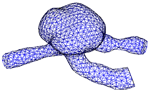
A DOLFIN mesh illustrating a patient-specific aneurysm geometry
To model blood flow we assume that blood is Newtonian and incompressible with a viscosity of 0.0035 Pa s and density similar to water. The equations read
Here, \(v\) and \(p\) are the unknown blood velocity and pressure, respectively, while \(\mu\) is the viscosity and \(\rho\) the density.
Quite often the outlet boundary conditions are unknown. It is therefore common to model the boundary conditions using differential equations of lower dimension. In our case, we assume that the pressure at the inlet or outlet boundaries can be modeled by a system of ODEs:
These ODEs are coupled to the Navier-Stokes equations through the inlet or outlet boundary condition
The FEniCS solver
The Navier-Stokes solver is implemented in FEniCS as a class NSSolver. The typical usage of the class goes as follows:
solver = NSSolver()
solver.setIC()
t = 0
dt = 0.01
T = 1.0
P1, P2 = 0, 0
while t < T:
    t += dt
    solver.advance_one_time_step((P1, P2), t)
The setIC() function sets the initial conditions. Futhermore, P1 and P2 are the pressures at the two outlets at time t. The implementation details of class NSSolver are not essential to this document, so we just refer the reader to the relatively short NSSolver.py file.
The Fortran code for modeling boundary conditions
The NSSolver class sets Dirichlet condition for the pressure on inlet and outlet boundaries in terms of prescribed constants in a list P (one for each prescribed outlet or inlet). Our aim now is to use a lower-dimensional flow model for computing the Dirichlet values in P based on physics and the current velocity and pressure fields. One such model is formulated in terms of ODEs. For an outlet boundary, let \(P\) be the pressure at the boundary. Then the model for \(P\) is
where
is the volume flux through the boundary \(\partial\Omega_o\) (easily computed in the FEniCS solver). The parameters \(C\) and \(R_d\) must be prescribed along with the initial value of \(P\).
The differential equation for \(P\) can be discretized by a very simple Forward Euler scheme. With \(i\) denoting the time level corresponding to small time steps \(\delta t\) in the fluid solver time step \(\Delta t\), we can write
for \(i=0,\ldots, N-1\), where \(\Delta t = N\delta t\), and then the new pressure outlet condition is \(P=P^{N}\) for the next time step. \(P^0\) is taken as \(P\) at time \(t\) (\(P\) is the outlet pressure value at time \(t+\Delta t\)).
The computational model for \(P\) is implemented in Fortran. (Our specific model is a simple one; the problem setting is that another research group is continuously developing such models, and their software is in Fortran.) The solver in Fortran is implemented in a file PMODEL.f with the content
      SUBROUTINE PMODEL(P, P_1, R_D, Q, C, N, T)
C     Integrate P in N steps from 0 to T, given start value P_1
      INTEGER N
      REAL*8 P(0:N), P_1, R_D, Q, C, T
      REAL*8 DT
      INTEGER I
Cf2py intent(in) P0, R, Q, C, N
Cf2py intent(out) P

      DT = T/N
      P(0) = P_1
      DO I = 0, N-1
        P(i+1) = P(i) + DT*(Q - P(i)/R_D)/C
      END DO
      END SUBROUTINE PMODEL
Given P_1 as the value of P at time t, the subroutine computes \(P\) at all the N local time steps (of length DT) up to time t+T, with P(N) as the final value at that time. We shall call PMODEL at every time step in the flow solver and let T correspond to the fluid solver time step \(\Delta t\).
The subroutine is plain Fortran 77 except for some special comment lines starting with CF2PY. These are needed because in Fortran, subroutine arguments are both input and output, but in Python one normally takes all input as arguments to a function and returns all output arguments. This is technically not possible in Fortran (or C or C++). With the CF2PY comment lines we can help the F2PY translater to make the Fortran subroutine look more “Pythonic” from the Python side. To this end, we need to specify what arguments that are input and output. All arguments are input by default, but here we still list them to have complete specification of every argument in this function. The output argument, to be returned to Python, must be specified, here P.
Creating a shared library of the Fortran code that we can call from Python as an ordinary module is easy:
Terminal> F2PY -c -m bcmodelf77 ../PMODEL.f
Here, -m bcmodelf77 tells F2PY that the module name is be bcmodelf77, the -c instructs F2PY to compile and create a shared library bcmodelf77.so, and PMODEL.f is the name of the Fortran file to analyze and compile. Our convention is to compile F2PY modules in a subdirectory of the Fortran code, which explains why the file here has name ../PMODEL.f.
A little test code can compare the Fortran ODE solver with a couple of manual lines in Python:
import nose.tools as nt

def test_bcmodelf77():
    import bcmodelf77
    C = 0.127
    R_d = 5.43
    N = 2
    P_1 = 16000
    Q = 1000
    T = 0.01
    P_ = bcmodelf77.pmodel(P_1, R_d, Q, C, N, T)

    # Manual formula:
    P1_ = P_1 + T/2*(Q - P_1/R_d)/C
    P1_ = P1_ + T/2*(Q - P1_/R_d)/C
    nt.assert_almost_equal(
        P_[-1], P1_, places=10, msg='F77: %g, manual coding: %s' %
        (P_[-1], P1_))

if __name__ == '__main__':
    test_bcmodelf77()
Note that F2PY turns all upper case letters into lower case when viewed from Python. Also note that this test function is created as a nose unit test. Running nosetests in that directory finds all test_* functions in all files and executes these functions.
Instead of calling the Fortran function directly with many parameters, we wrap a class around the function such that the syntax of each call to compute \(P\) becomes simpler. The idea is to let parameters that are constant through the fluid flow simulation be attributes in the class so that it is sufficient to provide the varying parameters in the call to PMODEL. The Python code hopefully explains this idea clearly:
class BCModel:
    def __init__(self, C, R_d, N, T):
        self.C, self.R, self.N, self.T = C, R_d, N, T

    def __call__(self, P, Q):
        P_ = bcmodelf77.pmodel(
             P, self.R, Q, self.C, self.N, self.T)
        return P_
We can now set all constant parameters at once,
pmodel = BCModel(C=0.127, R_d=5.43, N=2, T=0.01)
and there after call the Fortran subroutine PMODEL by pmodel(P, Q), i.e., with only the arguments that change from time step to time step in the fluid solver.
Coupling the Python FEniCS solver with the Fortran routine
It remains to make the final glue between the FEniCS solver and the Fortran subroutine. In the FEniCS solver, we import the BCModel class and make a list of such objects, with one element for each outlet boundary where we want to use the ODE model. Then we invoke a time loop where new \(u\) and \(p\) are computed, then we compute the flux \(Q\), and finally we compute new outlet pressures by calling up each ODE solver in turn. All this code is collected in the file CoupledSolver.py:
import NSSolver
from BCModel import BCModel

solver = NSSolver.NSSolver()
solver.setIC()
t = 0
dt = 0.01   # fluid solver time step
T = 5.0     # end time of simulation

C = 0.127
R = 5.43
N = 1000    # use N steps in the ODE solver in [t,t+dt]

num_outlets = 2  # no out outflow boundaries

# Create an ODE model for the pressure at each outlet boundary
pmodels = [BCModel(C, R, N, dt) for i in range(0,num_outlets)]

P_ = [16000, 100]   # start values for outlet pressures

while t < T:
    t += dt

    # Compute u_ and p_ using known outlet pressures P_
    solver.advance_one_time_step(P_, t)
    # Compute the flux at outlet boundaries
    Q = solver.flux()

    # Advance outlet pressure boundary condition to the
    # next time step (for each outlet boundary)
    # (pmodels returns a vector of size N containg the
    # the solution between [t, t+dt].
    # We take the last one with [-1])
    for i in range(0, num_outlets):
        P_[i] = pmodels[i](P_[i], Q[i])[-1]
