Applications of wave equations

This section presents a range of wave equation models for different physical phenomena. Although many wave motion problems in physics can be modeled by the standard linear wave equation, or a similar formulation with a system of first-order equations, there are some exceptions. Perhaps the most important is water waves: these are modeled by the Laplace equation with time-dependent boundary conditions at the water surface (long water waves, however, can be approximated by a standard wave equation, see the section The linear shallow water equations). Quantum mechanical waves constitute another example where the waves are governed by the Schrodinger equation, i.e., not by a standard wave equation. Many wave phenomena also need to take nonlinear effects into account when the wave amplitude is significant. Shock waves in the air is a primary example.

The derivations in the following are very brief. Those with a firm background in continuum mechanics will probably have enough knowledge to fill in the details, while other readers will hopefully get some impression of the physics and approximations involved when establishing wave equation models.

Waves on a string

Figure 33: Discrete string model with point masses connected by elastic strings.

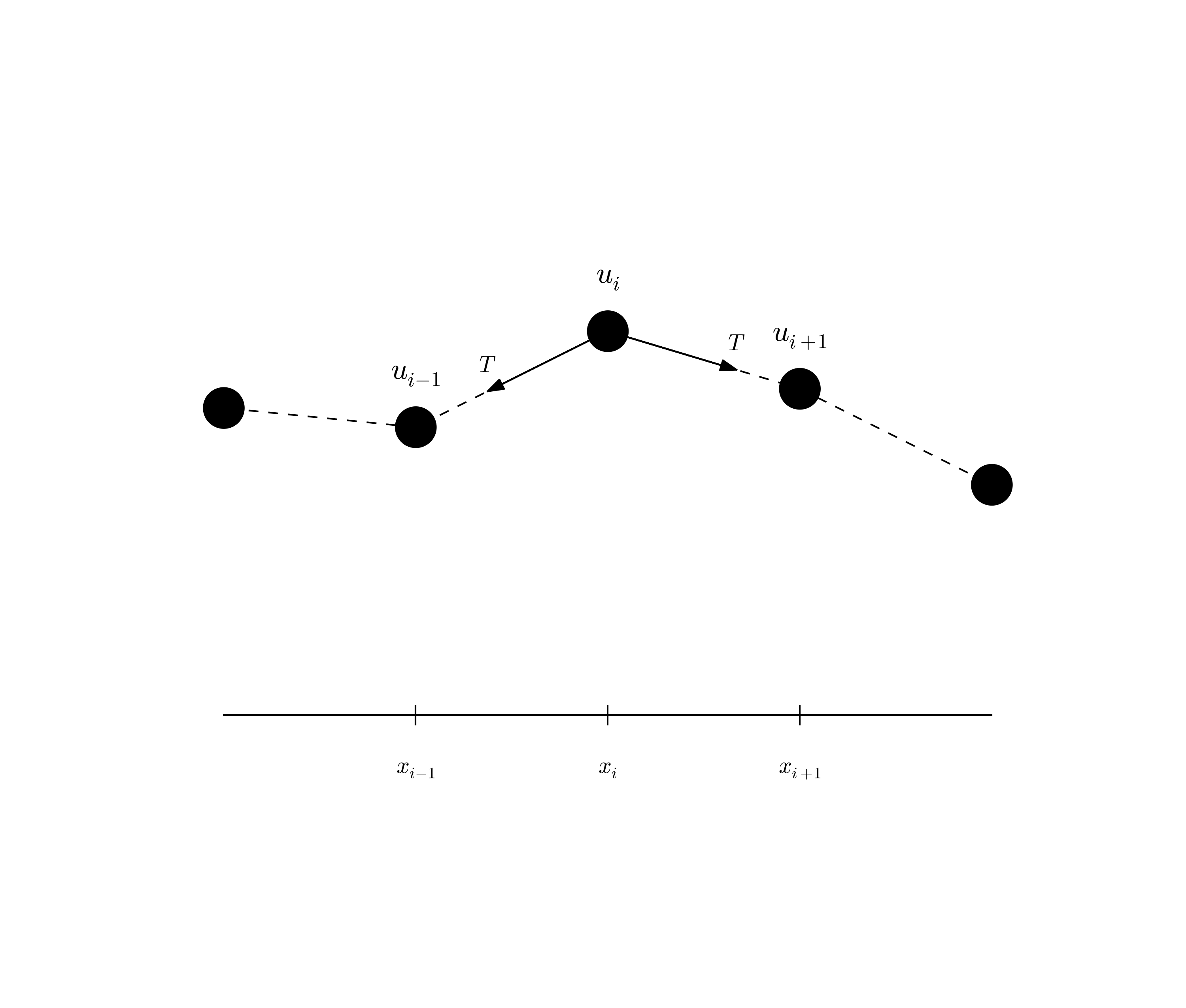
Figure 33 shows a model we may use to derive the equation for waves on a string. The string is modeled as a set of discrete point masses (at mesh points) with elastic strings in between. The string has a large constant tension $ T $. We let the mass at mesh point $ x_i $ be $ m_i $. The displacement of this mass point in the $ y $ direction is denoted by $ u_i(t) $.

The motion of mass $ m_i $ is governed by Newton's second law of motion. The position of the mass at time $ t $ is $ x_i\ii + u_i(t)\jj $, where $ \ii $ and $ \jj $ are unit vectors in the $ x $ and $ y $ direction, respectively. The acceleration is then $ u_i''(t)\jj $. Two forces are acting on the mass as indicated in Figure 33. The force $ \T^{-} $ acting toward the point $ x_{i-1} $ can be decomposed as $$ \T^{-} = -T\sin\phi\ii -T\cos\phi\jj, $$ where $ \phi $ is the angle between the force and the line $ x=x_i $. Let $ \Delta u_i = u_i - u_{i-1} $ and let $ \Delta s_i = \sqrt{\Delta u_i^2 + (x_i - x_{i-1})^2} $ be the distance from mass $ m_{i-1} $ to mass $ m_i $. It is seen that $ \cos\phi = \Delta u_i/\Delta s_i $ and $ \sin\phi = (x_{i}-x_{i-1})/\Delta s $ or $ \Delta x/\Delta s_i $ if we introduce a constant mesh spacing $ \Delta x = x_i - x_{i-1} $. The force can then be written $$ \T^{-} = -T\frac{\Delta x}{\Delta s_i}\ii - T\frac{\Delta u_i}{\Delta s_i}\jj \tp $$ The force $ \T^{+} $ acting toward $ x_{i+1} $ can be calculated in a similar way: $$ \T^{+} = T\frac{\Delta x}{\Delta s_{i+1}}\ii + T\frac{\Delta u_{i+1}}{\Delta s_{i+1}}\jj \tp $$ Newton's second law becomes $$ m_iu_i''(t)\jj = \T^{+} + \T^{-},$$ which gives the component equations $$ \begin{align} T\frac{\Delta x}{\Delta s_i} &= T\frac{\Delta x}{\Delta s_{i+1}}, \tag{2.116}\\ m_iu_i''(t) &= T\frac{\Delta u_{i+1}}{\Delta s_{i+1}} - T\frac{\Delta u_i}{\Delta s_i} \tag{2.117} \tp \end{align} $$

A basic reasonable assumption for a string is small displacements $ u_i $ and small displacement gradients $ \Delta u_i/\Delta x $. For small $ g=\Delta u_i/\Delta x $ we have that $$ \Delta s_i = \sqrt{\Delta u_i^2 + \Delta x^2} = \Delta x\sqrt{1 + g^2} + \Delta x (1 + {\half}g^2 + {\cal O}(g^4) \approx \Delta x \tp $$ Equation (2.116) is then simply the identity $ T=T $, while (2.117) can be written as $$ m_iu_i''(t) = T\frac{\Delta u_{i+1}}{\Delta x} - T\frac{\Delta u_i}{\Delta x}, $$ which upon division by $ \Delta x $ and introducing the density $ \varrho_i = m_i/\Delta x $ becomes $$ \begin{equation} \varrho_i u_i''(t) = T\frac{1}{\Delta x^2} \left( u_{i+1} - 2u_i + u_{i-1}\right) \tag{2.118} \tp \end{equation} $$ We can now choose to approximate $ u_i'' $ by a finite difference in time and get the discretized wave equation, $$ \begin{equation} \varrho_i \frac{1}{\Delta t^2} \left(u^{n+1}_i - 2u^n_i - u^{n-1}_i\right) = T\frac{1}{\Delta x^2} \left( u_{i+1} - 2u_i + u_{i-1}\right)\tp \tag{2.119} \end{equation} $$ On the other hand, we may go to the continuum limit $ \Delta x\rightarrow 0 $ and replace $ u_i(t) $ by $ u(x,t) $, $ \varrho_i $ by $ \varrho(x) $, and recognize that the right-hand side of (2.118) approaches $ \partial^2 u/\partial x^2 $ as $ \Delta x\rightarrow 0 $. We end up with the continuous model for waves on a string: $$ \begin{equation} \varrho\frac{\partial^2 u}{\partial t^2} = T\frac{\partial^2 u}{\partial x^2} \tag{2.120} \tp \end{equation} $$ Note that the density $ \varrho $ may change along the string, while the tension $ T $ is a constant. With variable wave velocity $ c(x) = \sqrt{T/\varrho(x)} $ we can write the wave equation in the more standard form $$ \begin{equation} \frac{\partial^2 u}{\partial t^2} = c^2(x)\frac{\partial^2 u}{\partial x^2} \tag{2.121} \tp \end{equation} $$ Because of the way $ \varrho $ enters the equations, the variable wave velocity does not appear inside the derivatives as in many other versions of the wave equation. However, most strings of interest have constant $ \varrho $.

The end points of a string are fixed so that the displacement $ u $ is zero. The boundary conditions are therefore $ u=0 $.

Damping

Air resistance and non-elastic effects in the string will contribute to reduce the amplitudes of the waves so that the motion dies out after some time. This damping effect can be modeled by a term $ bu_t $ on the left-hand side of the equation $$ \begin{equation} \varrho\frac{\partial^2 u}{\partial t^2} + b\frac{\partial u}{\partial t} = T\frac{\partial^2 u}{\partial x^2} \tag{2.122} \tp \end{equation} $$ The parameter $ b\geq 0 $ is small for most wave phenomena, but the damping effect may become significant in long time simulations.

External forcing

It is easy to include an external force acting on the string. Say we have a vertical force $ \tilde f_i\jj $ acting on mass $ m_i $, modeling the effect of gravity on a string. This force affects the vertical component of Newton's law and gives rise to an extra term $ \tilde f(x,t) $ on the right-hand side of (2.120). In the model (2.121) we would add a term $ f(x,t) = \tilde f(x,t)/\varrho(x) $.

Modeling the tension via springs

We assumed, in the derivation above, that the tension in the string, $ T $, was constant. It is easy to check this assumption by modeling the string segments between the masses as standard springs, where the force (tension $ T $) is proportional to the elongation of the spring segment. Let $ k $ be the spring constant, and set $ T_i=k\Delta \ell $ for the tension in the spring segment between $ x_{i-1} $ and $ x_i $, where $ \Delta\ell $ is the elongation of this segment from the tension-free state. A basic feature of a string is that it has high tension in the equilibrium position $ u=0 $. Let the string segment have an elongation $ \Delta\ell_0 $ in the equilibrium position. After deformation of the string, the elongation is $ \Delta \ell = \Delta \ell_0 + \Delta s_i $: $ T_i = k(\Delta \ell_0 + \Delta s_i)\approx k(\Delta \ell_0 + \Delta x) $. This shows that $ T_i $ is independent of $ i $. Moreover, the extra approximate elongation $ \Delta x $ is very small compared to $ \Delta\ell_0 $, so we may well set $ T_i = T = k\Delta\ell_0 $. This means that the tension is completely dominated by the initial tension determined by the tuning of the string. The additional deformations of the spring during the vibrations do not introduce significant changes in the tension.

Elastic waves in a rod

Consider an elastic rod subject to a hammer impact at the end. This experiment will give rise to an elastic deformation pulse that travels through the rod. A mathematical model for longitudinal waves along an elastic rod starts with the general equation for deformations and stresses in an elastic medium, $$ \begin{equation} \varrho\u_{tt} = \nabla\cdot\stress + \varrho\f, \tag{2.123} \end{equation} $$ where $ \varrho $ is the density, $ \u $ the displacement field, $ \stress $ the stress tensor, and $ \f $ body forces. The latter has normally no impact on elastic waves.

For stationary deformation of an elastic rod, aligned with the $ x $ axis, one has that $ \sigma_{xx} = Eu_x $, with all other stress components being zero. The parameter $ E $ is known as Young's modulus. Moreover, we set $ \u = u(x,t)\ii $ and neglect the radial contraction and expansion (where Poisson's ratio is the important parameter). Assuming that this simple stress and deformation field is a good approximation, (2.123) simplifies to $$ \begin{equation} \varrho\frac{\partial^2 u}{\partial t^2} = \frac{\partial}{\partial x} \left( E\frac{\partial u}{\partial x}\right) \tag{2.124} \tp \end{equation} $$

The associated boundary conditions are $ u $ or $ \sigma_{xx}=Eu_x $ known, typically $ u=0 $ for a fixed end and $ \sigma_{xx}=0 $ for a free end.

Waves on a membrane

Think of a thin, elastic membrane with shape as a circle or rectangle. This membrane can be brought into oscillatory motion and will develop elastic waves. We can model this phenomenon somewhat similar to waves in a rod: waves in a membrane are simply the two-dimensional counterpart. We assume that the material is deformed in the $ z $ direction only and write the elastic displacement field on the form $ \u (x,y,t) = w(x,y,t)\ii $. The $ z $ coordinate is omitted since the membrane is thin and all properties are taken as constant throughout the thickness. Inserting this displacement field in Newton's 2nd law of motion (2.123) results in $$ \begin{equation} \varrho\frac{\partial^2 w}{\partial t^2} = \frac{\partial}{\partial x} \left( \mu\frac{\partial w}{\partial x}\right) + \frac{\partial}{\partial y} \left( \mu\frac{\partial w}{\partial y}\right) \tag{2.125} \tp \end{equation} $$ This is nothing but a wave equation in $ w(x,y,t) $, which needs the usual initial conditions on $ w $ and $ w_t $ as well as a boundary condition $ w=0 $. When computing the stress in the membrane, one needs to split $ \stress $ into a constant high-stress component due to the fact that all membranes are normally pre-stressed, plus a component proportional to the displacement and governed by the wave motion.

The acoustic model for seismic waves

Seismic waves are used to infer properties of subsurface geological structures. The physical model is a heterogeneous elastic medium where sound is propagated by small elastic vibrations. The general mathematical model for deformations in an elastic medium is based on Newton's second law, $$ \begin{equation} \varrho\u_{tt} = \nabla\cdot\stress + \varrho\f, \tag{2.126} \end{equation} $$ and a constitutive law relating $ \stress $ to $ \u $, often Hooke's generalized law, $$ \begin{equation} \stress = K\nabla\cdot\u\, \I + G(\nabla\u + (\nabla\u)^T - \frac{2}{3}\nabla\cdot\u\, \I) \tag{2.127} \tp \end{equation} $$ Here, $ \u $ is the displacement field, $ \stress $ is the stress tensor, $ \I $ is the identity tensor, $ \varrho $ is the medium's density, $ \f $ are body forces (such as gravity), $ K $ is the medium's bulk modulus and $ G $ is the shear modulus. All these quantities may vary in space, while $ \u $ and $ \stress $ will also show significant variation in time during wave motion.

The acoustic approximation to elastic waves arises from a basic assumption that the second term in Hooke's law, representing the deformations that give rise to shear stresses, can be neglected. This assumption can be interpreted as approximating the geological medium by a fluid. Neglecting also the body forces $ \f $, (2.126) becomes $$ \begin{equation} \varrho\u_{tt} = \nabla (K\nabla\cdot\u ) \tag{2.128} \end{equation} $$ Introducing $ p $ as a pressure via $$ \begin{equation} p=-K\nabla\cdot\u, \tag{2.129} \end{equation} $$ and dividing (2.128) by $ \varrho $, we get $$ \begin{equation} \u_{tt} = -\frac{1}{\varrho}\nabla p \tp \tag{2.130} \end{equation} $$ Taking the divergence of this equation, using $ \nabla\cdot\u = -p/K $ from (2.129), gives the acoustic approximation to elastic waves: $$ \begin{equation} p_{tt} = K\nabla\cdot\left(\frac{1}{\varrho}\nabla p\right) \tp \tag{2.131} \end{equation} $$ This is a standard, linear wave equation with variable coefficients. It is common to add a source term $ s(x,y,z,t) $ to model the generation of sound waves: $$ \begin{equation} p_{tt} = K\nabla\cdot\left(\frac{1}{\varrho}\nabla p\right) + s \tp \tag{2.132} \end{equation} $$

A common additional approximation of (2.132) is based on using the chain rule on the right-hand side, $$ K\nabla\cdot\left(\frac{1}{\varrho}\nabla p\right) = \frac{K}{\varrho}\nabla^2 p + K\nabla\left(\frac{1}{\varrho}\right)\cdot \nabla p \approx \frac{K}{\varrho}\nabla^2 p, $$ under the assumption that the relative spatial gradient $ \nabla\varrho^{-1} = -\varrho^{-2}\nabla\varrho $ is small. This approximation results in the simplified equation $$ \begin{equation} p_{tt} = \frac{K}{\varrho}\nabla^2 p + s \tp \tag{2.133} \end{equation} $$

The acoustic approximations to seismic waves are used for sound waves in the ground, and the Earth's surface is then a boundary where $ p $ equals the atmospheric pressure $ p_0 $ such that the boundary condition becomes $ p=p_0 $.

Anisotropy

Quite often in geological materials, the effective wave velocity $ c=\sqrt{K/\varrho} $ is different in different spatial directions because geological layers are compacted, and often twisted, in such a way that the properties in the horizontal and vertical direction differ. With $ z $ as the vertical coordinate, we can introduce a vertical wave velocity $ c_z $ and a horizontal wave velocity $ c_h $, and generalize (2.133) to $$ \begin{equation} p_{tt} = c_z^2 p_{zz} + c_h^2 (p_{xx} + p_{yy}) + s \tp \tag{2.134} \end{equation} $$

Sound waves in liquids and gases

Sound waves arise from pressure and density variations in fluids. The starting point of modeling sound waves is the basic equations for a compressible fluid where we omit viscous (frictional) forces, body forces (gravity, for instance), and temperature effects: $$ \begin{align} \varrho_t + \nabla\cdot (\varrho \u) &= 0, \tag{2.135}\\ \varrho \u_{t} + \varrho \u\cdot\nabla\u &= -\nabla p, \tag{2.136}\\ \varrho &= \varrho (p) \tp \tag{2.137} \end{align} $$ These equations are often referred to as the Euler equations for the motion of a fluid. The parameters involved are the density $ \varrho $, the velocity $ \u $, and the pressure $ p $. Equation reflects (2.135) mass balance, (2.136) is Newton's second law for a fluid, with frictional and body forces omitted, and (2.137) is a constitutive law relating density to pressure by thermodynamic considerations. A typical model for (2.137) is the so-called isentropic relation, valid for adiabatic processes where there is no heat transfer: $$ \begin{equation} \varrho = \varrho_0\left(\frac{p}{p_0}\right)^{1/\gamma} \tp \tag{2.138} \end{equation} $$ Here, $ p_0 $ and $ \varrho_0 $ are reference values for $ p $ and $ \varrho $ when the fluid is at rest, and $ \gamma $ is the ratio of specific heat at constant pressure and constant volume ($ \gamma = 5/3 $ for air).

The key approximation in a mathematical model for sound waves is to assume that these waves are small perturbations to the density, pressure, and velocity. We therefore write $$ \begin{align*} p &= p_0 + \hat p,\\ \varrho &= \varrho_0 + \hat\varrho,\\ \u &= \hat\u, \end{align*} $$ where we have decomposed the fields in a constant equilibrium value, corresponding to $ \u=0 $, and a small perturbation marked with a hat symbol. By inserting these decompositions in (2.135) and (2.136), neglecting all product terms of small perturbations and/or their derivatives, and dropping the hat symbols, one gets the following linearized PDE system for the small perturbations in density, pressure, and velocity: $$ \begin{align} \varrho_t + \varrho_0\nabla\cdot\u &= 0, \tag{2.139}\\ \varrho_0\u_t &= -\nabla p \tp \tag{2.140} \end{align} $$ Now we can eliminate $ \varrho_t $ by differentiating the relation $ \varrho(p) $, $$ \varrho_t = \varrho_0 \frac{1}{\gamma}\left(\frac{p}{p_0}\right)^{1/\gamma-1} \frac{1}{p_0}p_t = \frac{\varrho_0}{\gamma p_0} \left(\frac{p}{p_0}\right)^{1/\gamma-1}p_t \tp $$ The product term $ p^{1/\gamma -1}p_t $ can be linearized as $ p_0^{1/\gamma -1}p_t $, resulting in $$ \varrho_t \approx \frac{\varrho_0}{\gamma p_0} p_t \tp $$ We then get $$ \begin{align} p_t + \gamma p_0\nabla\cdot\u &= 0, \tag{2.141}\\ \u_t &= -\frac{1}{\varrho_0}\nabla p, \tag{2.142} \tp \end{align} $$ Taking the divergence of (2.142) and differentiating (2.141) with respect to time gives the possibility to easily eliminate $ \nabla\cdot\u_t $ and arrive at a standard, linear wave equation for $ p $: $$ \begin{equation} p_{tt} = c^2\nabla^2 p, \tag{2.143} \end{equation} $$ where $ c = \sqrt{\gamma p_0/\varrho_0} $ is the speed of sound in the fluid.

Spherical waves

Spherically symmetric three-dimensional waves propagate in the radial direction $ r $ only so that $ u = u(r,t) $. The fully three-dimensional wave equation $$ \frac{\partial^2u}{\partial t^2}=\nabla\cdot (c^2\nabla u) + f $$ then reduces to the spherically symmetric wave equation $$ \begin{equation} \frac{\partial^2u}{\partial t^2}=\frac{1}{r^2}\frac{\partial}{\partial r} \left(c^2(r)r^2\frac{\partial u}{\partial r}\right) + f(r,t),\quad r\in (0,R),\ t>0 \tp \tag{2.144} \end{equation} $$ One can easily show that the function $ v(r,t) = ru(r,t) $ fulfills a standard wave equation in Cartesian coordinates if $ c $ is constant. To this end, insert $ u=v/r $ in $$ \frac{1}{r^2}\frac{\partial}{\partial r} \left(c^2(r)r^2\frac{\partial u}{\partial r}\right) $$ to obtain $$ r\left(\frac{d c^2}{dr}\frac{\partial v}{\partial r} + c^2\frac{\partial^2 v}{\partial r^2}\right) - \frac{d c^2}{dr}v \tp $$ The two terms in the parenthesis can be combined to $$ r\frac{\partial}{\partial r}\left( c^2\frac{\partial v}{\partial r}\right), $$ which is recognized as the variable-coefficient Laplace operator in one Cartesian coordinate. The spherically symmetric wave equation in terms of $ v(r,t) $ now becomes $$ \begin{equation} \frac{\partial^2v}{\partial t^2}= \frac{\partial}{\partial r} \left(c^2(r)\frac{\partial v}{\partial r}\right) -\frac{1}{r}\frac{d c^2}{dr}v + rf(r,t),\quad r\in (0,R),\ t>0 \tp \tag{2.145} \end{equation} $$ In the case of constant wave velocity $ c $, this equation reduces to the wave equation in a single Cartesian coordinate called $ r $: $$ \begin{equation} \frac{\partial^2v}{\partial t^2}= c^2 \frac{\partial^2 v}{\partial r^2} + rf(r,t),\quad r\in (0,R),\ t>0 \tp \tag{2.146} \end{equation} $$ That is, any program for solving the one-dimensional wave equation in a Cartesian coordinate system can be used to solve (2.146), provided the source term is multiplied by the coordinate, and that we divide the Cartesian mesh solution by $ r $ to get the spherically symmetric solution. Moreover, if $ r=0 $ is included in the domain, spherical symmetry demands that $ \partial u/\partial r=0 $ at $ r=0 $, which means that $$ \frac{\partial u}{\partial r} = \frac{1}{r^2}\left( r\frac{\partial v}{\partial r} - v\right) = 0,\quad r=0\tp $$ For this to hold in the limit $ r\rightarrow 0 $, we must have $ v(0,t)=0 $ at least as a necessary condition. In most practical applications, we exclude $ r=0 $ from the domain and assume that some boundary condition is assigned at $ r=\epsilon $, for some $ \epsilon >0 $.

The linear shallow water equations

The next example considers water waves whose wavelengths are much larger than the depth and whose wave amplitudes are small. This class of waves may be generated by catastrophic geophysical events, such as earthquakes at the sea bottom, landslides moving into water, or underwater slides (or a combination, as earthquakes frequently release avalanches of masses). For example, a subsea earthquake will normally have an extension of many kilometers but lift the water only a few meters. The wave length will have a size dictated by the earthquake area, which is much lager than the water depth, and compared to this wave length, an amplitude of a few meters is very small. The water is essentially a thin film, and mathematically we can average the problem in the vertical direction and approximate the 3D wave phenomenon by 2D PDEs. Instead of a moving water domain in three space dimensions, we get a horizontal 2D domain with an unknown function for the surface elevation and the water depth as a variable coefficient in the PDEs.

Let $ \eta(x,y,t) $ be the elevation of the water surface, $ H(x,y) $ the water depth corresponding to a flat surface ($ \eta =0 $), $ u(x,y,t) $ and $ v(x,y,t) $ the depth-averaged horizontal velocities of the water. Mass and momentum balance of the water volume give rise to the PDEs involving these quantities: $$ \begin{align} \eta_t &= - (Hu)_x - (Hv)_x \tag{2.147}\\ u_t &= -g\eta_x, \tag{2.148}\\ v_t &= -g\eta_y, \tag{2.149} \end{align} $$ where $ g $ is the acceleration of gravity. Equation (2.147) corresponds to mass balance while the other two are derived from momentum balance (Newton's second law).

The initial conditions associated with (2.147)-(2.149) are $ \eta $, $ u $, and $ v $ prescribed at $ t=0 $. A common condition is to have some water elevation $ \eta =I(x,y) $ and assume that the surface is at rest: $ u=v=0 $. A subsea earthquake usually means a sufficiently rapid motion of the bottom and the water volume to say that the bottom deformation is mirrored at the water surface as an initial lift $ I(x,y) $ and that $ u=v=0 $.

Boundary conditions may be $ \eta $ prescribed for incoming, known waves, or zero normal velocity at reflecting boundaries (steep mountains, for instance): $ un_x + vn_y =0 $, where $ (n_x,n_y) $ is the outward unit normal to the boundary. More sophisticated boundary conditions are needed when waves run up at the shore, and at open boundaries where we want the waves to leave the computational domain undisturbed.

Equations (2.147), (2.148), and (2.149) can be transformed to a standard, linear wave equation. First, multiply (2.148) and (2.149) by $ H $, differentiate (2.148)) with respect to $ x $ and (2.149) with respect to $ y $. Second, differentiate (2.147) with respect to $ t $ and use that $ (Hu)_{xt}=(Hu_t)_x $ and $ (Hv)_{yt}=(Hv_t)_y $ when $ H $ is independent of $ t $. Third, eliminate $ (Hu_t)_x $ and $ (Hv_t)_y $ with the aid of the other two differentiated equations. These manipulations result in a standard, linear wave equation for $ \eta $: $$ \begin{equation} \eta_{tt} = (gH\eta_x)_x + (gH\eta_y)_y = \nabla\cdot (gH\nabla\eta) \tag{2.150} \tp \end{equation} $$

In the case we have an initial non-flat water surface at rest, the initial conditions become $ \eta =I(x,y) $ and $ \eta_t=0 $. The latter follows from (2.147) if $ u=v=0 $, or simply from the fact that the vertical velocity of the surface is $ \eta_t $, which is zero for a surface at rest.

The system (2.147)-(2.149) can be extended to handle a time-varying bottom topography, which is relevant for modeling long waves generated by underwater slides. In such cases the water depth function $ H $ is also a function of $ t $, due to the moving slide, and one must add a time-derivative term $ H_t $ to the left-hand side of (2.147). A moving bottom is best described by introducing $ z=H_0 $ as the still-water level, $ z=B(x,y,t) $ as the time- and space-varying bottom topography, so that $ H=H_0-B(x,y,t) $. In the elimination of $ u $ and $ v $ one may assume that the dependence of $ H $ on $ t $ can be neglected in the terms $ (Hu)_{xt} $ and $ (Hv)_{yt} $. We then end up with a source term in (2.150), because of the moving (accelerating) bottom: $$ \begin{equation} \eta_{tt} = \nabla\cdot(gH\nabla\eta) + B_{tt} \tag{2.151} \tp \end{equation} $$

The reduction of (2.151) to 1D, for long waves in a straight channel, or for approximately plane waves in the ocean, is trivial by assuming no change in $ y $ direction ($ \partial/\partial y=0 $): $$ \begin{equation} \eta_{tt} = (gH\eta_x)_x + B_{tt} \tag{2.152} \tp \end{equation} $$

Wind drag on the surface

Surface waves are influenced by the drag of the wind, and if the wind velocity some meters above the surface is $ (U,V) $, the wind drag gives contributions $ C_V\sqrt{U^2+V^2}U $ and $ C_V\sqrt{U^2+V^2}V $ to (2.148) and (2.149), respectively, on the right-hand sides.

Bottom drag

The waves will experience a drag from the bottom, often roughly modeled by a term similar to the wind drag: $ C_B\sqrt{u^2+v^2}u $ on the right-hand side of (2.148) and $ C_B\sqrt{u^2+v^2}v $ on the right-hand side of (2.149). Note that in this case the PDEs (2.148) and (2.149) become nonlinear and the elimination of $ u $ and $ v $ to arrive at a 2nd-order wave equation for $ \eta $ is not possible anymore.

Effect of the Earth's rotation

Long geophysical waves will often be affected by the rotation of the Earth because of the Coriolis force. This force gives rise to a term $ fv $ on the right-hand side of (2.148) and $ -fu $ on the right-hand side of (2.149). Also in this case one cannot eliminate $ u $ and $ v $ to work with a single equation for $ \eta $. The Coriolis parameter is $ f=2\Omega\sin\phi $, where $ \Omega $ is the angular velocity of the earth and $ \phi $ is the latitude.

Waves in blood vessels

The flow of blood in our bodies is basically fluid flow in a network of pipes. Unlike rigid pipes, the walls in the blood vessels are elastic and will increase their diameter when the pressure rises. The elastic forces will then push the wall back and accelerate the fluid. This interaction between the flow of blood and the deformation of the vessel wall results in waves traveling along our blood vessels.

A model for one-dimensional waves along blood vessels can be derived from averaging the fluid flow over the cross section of the blood vessels. Let $ x $ be a coordinate along the blood vessel and assume that all cross sections are circular, though with different radii $ R(x,t) $. The main quantities to compute is the cross section area $ A(x,t) $, the averaged pressure $ P(x,t) $, and the total volume flux $ Q(x,t) $. The area of this cross section is $$ \begin{equation} A(x,t) = 2\pi\int_{0}^{R(x,t)} rdr, \tag{2.153} \end{equation} $$ Let $ v_x(x,t) $ be the velocity of blood averaged over the cross section at point $ x $. The volume flux, being the total volume of blood passing a cross section per time unit, becomes $$ \begin{equation} Q(x,t) = A(x,t)v_x(x,t) \thinspace \tag{2.154} \end{equation} $$

Mass balance and Newton's second law lead to the PDEs $$ \begin{align} \frac{\partial A}{\partial t} + \frac{\partial Q}{\partial x} &= 0, \tag{2.155}\\ \frac{\partial Q}{\partial t} + \frac{\gamma+2}{\gamma + 1} \frac{\partial}{\partial x}\left(\frac{Q^2}{A}\right) + \frac{A}{\varrho}\frac{\partial P}{\partial x} &= -2\pi (\gamma + 2)\frac{\mu}{\varrho}\frac{Q}{A}, \tag{2.156} \end{align} $$ where $ \gamma $ is a parameter related to the velocity profile, $ \varrho $ is the density of blood, and $ \mu $ is the dynamic viscosity of blood.

We have three unknowns $ A $, $ Q $, and $ P $, and two equations (2.155) and (2.156). A third equation is needed to relate the flow to the deformations of the wall. A common form for this equation is $$ \begin{equation} \frac{\partial P}{\partial t} + \frac{1}{C} \frac{\partial Q}{\partial x} =0, \tag{2.157} \end{equation} $$ where $ C $ is the compliance of the wall, given by the constitutive relation $$ \begin{equation} C = \frac{\partial A}{\partial P} + \frac{\partial A}{\partial t}, \tag{2.158} \end{equation} $$ which requires a relationship between $ A $ and $ P $. One common model is to view the vessel wall, locally, as a thin elastic tube subject to an internal pressure. This gives the relation $$ P=P_0 + \frac{\pi h E}{(1-\nu^2)A_0}(\sqrt{A} - \sqrt{A_0}), $$ where $ P_0 $ and $ A_0 $ are corresponding reference values when the wall is not deformed, $ h $ is the thickness of the wall, and $ E $ and $ \nu $ are Young's modulus and Poisson's ratio of the elastic material in the wall. The derivative becomes $$ \begin{equation} C = \frac{\partial A}{\partial P} = \frac{2(1-\nu^2)A_0}{\pi h E}\sqrt{A_0} + 2\left(\frac{(1-\nu^2)A_0}{\pi h E}\right)^2(P-P_0) \tp \tag{2.159} \end{equation} $$ Another (nonlinear) deformation model of the wall, which has a better fit with experiments, is $$ P = P_0\exp{(\beta (A/A_0 - 1))},$$ where $ \beta $ is some parameter to be estimated. This law leads to $$ \begin{equation} C = \frac{\partial A}{\partial P} = \frac{A_0}{\beta P} \tp \tag{2.160} \end{equation} $$

Reduction to the standard wave equation. It is not uncommon to neglect the viscous term on the right-hand side of (2.156) and also the quadratic term with $ Q^2 $ on the left-hand side. The reduced equations (2.156) and (2.157) form a first-order linear wave equation system: $$ \begin{align} C\frac{\partial P}{\partial t} &= - \frac{\partial Q}{\partial x}, \tag{2.161}\\ \frac{\partial Q}{\partial t} &= - \frac{A}{\varrho}\frac{\partial P}{\partial x} \tp \tag{2.162} \end{align} $$ These can be combined into standard 1D wave PDE by differentiating the first equation with respect to $ t $ and the second with respect to $ x $, $$ \frac{\partial}{\partial t}\left( C\frac{\partial P}{\partial t} \right) = \frac{\partial}{\partial x}\left( \frac{A}{\varrho}\frac{\partial P}{\partial x}\right),$$ which can be approximated by $$ \begin{equation} \frac{\partial^2 Q}{\partial t^2} = c^2\frac{\partial^2 Q}{\partial x^2},\quad c = \sqrt{\frac{A}{\varrho C}}, \tag{2.163} \end{equation} $$ where the $ A $ and $ C $ in the expression for $ c $ are taken as constant reference values.

Electromagnetic waves

Light and radio waves are governed by standard wave equations arising from Maxwell's general equations. When there are no charges and no currents, as in a vacuum, Maxwell's equations take the form $$ \begin{align*} \nabla\cdot\pmb{E} &= 0,\\ \nabla\cdot\pmb{B} &= 0,\\ \nabla\times\pmb{E} &= -\frac{\partial\pmb{B}}{\partial t},\\ \nabla\times\pmb{B} &= \mu_0\epsilon_0\frac{\partial\pmb{E}}{\partial t}, \end{align*} $$ where $ \epsilon_0=8.854187817620\cdot 10^{-12} $ (F/m) is the permittivity of free space, also known as the electric constant, and $ \mu_0=1.2566370614\cdot 10^{-6} $ (H/m) is the permeability of free space, also known as the magnetic constant. Taking the curl of the two last equations and using the mathematical identity $$ \nabla\times (\nabla\times \pmb{E}) = \nabla(\nabla \cdot \pmb{E}) - \nabla^2\pmb{E} = - \nabla^2\pmb{E}\hbox{ when }\nabla\cdot\pmb{E}=0, $$ gives the wave equation governing the electric and magnetic field: $$ \begin{align} \frac{\partial^2\pmb{E}}{\partial t^2} &= c^2\nabla^2\pmb{E}, \tag{2.164}\\ \frac{\partial^2\pmb{B}}{\partial t^2} &= c^2\nabla^2\pmb{B}, \tag{2.165} \end{align} $$ with $ c=1/\sqrt{\mu_0\epsilon_0} $ as the velocity of light. Each component of $ \pmb{E} $ and $ \pmb{B} $ fulfills a wave equation and can hence be solved independently.