Finite difference methods for 2D and 3D wave equations
A natural next step is to consider extensions of the methods for various variants of the one-dimensional wave equation to two-dimensional (2D) and three-dimensional (3D) versions of the wave equation.
Multi-dimensional wave equations
The general wave equation in \( d \) space dimensions, with constant wave velocity \( c \), can be written in the compact form $$ \begin{equation} \frac{\partial^2 u}{\partial t^2} = c^2\nabla^2 u\hbox{ for }\xpoint\in\Omega\subset\Real^d,\ t\in (0,T] , \tag{2.104} \end{equation} $$ where $$ \begin{equation*} \nabla^2 u = \frac{\partial^2 u}{\partial x^2} + \frac{\partial^2 u}{\partial y^2} ,\end{equation*} $$ in a 2D problem (\( d=2 \)) and $$ \begin{equation*} \nabla^2 u = \frac{\partial^2 u}{\partial x^2} + \frac{\partial^2 u}{\partial y^2} + \frac{\partial^2 u}{\partial z^2}, \end{equation*} $$ in three space dimensions (\( d=3 \)).
Many applications involve variable coefficients, and the general wave equation in \( d \) dimensions is in this case written as $$ \begin{equation} \varrho\frac{\partial^2 u}{\partial t^2} = \nabla\cdot (q\nabla u) + f\hbox{ for }\xpoint\in\Omega\subset\Real^d,\ t\in (0,T], \tag{2.105} \end{equation} $$ which in, e.g., 2D becomes $$ \begin{equation} \varrho(x,y) \frac{\partial^2 u}{\partial t^2} = \frac{\partial}{\partial x}\left( q(x,y) \frac{\partial u}{\partial x}\right) + \frac{\partial}{\partial y}\left( q(x,y) \frac{\partial u}{\partial y}\right) + f(x,y,t) \tp \tag{2.106} \end{equation} $$ To save some writing and space we may use the index notation, where subscript \( t \), \( x \), or \( y \) means differentiation with respect to that coordinate. For example, $$ \begin{align*} \frac{\partial^2 u}{\partial t^2} &= u_{tt},\\ \frac{\partial}{\partial y}\left( q(x,y) \frac{\partial u}{\partial y}\right) &= (q u_y)_y \tp \end{align*} $$ These comments extend straightforwardly to 3D, which means that the 3D versions of the two wave PDEs, with and without variable coefficients, can be stated as $$ \begin{align} u_{tt} &= c^2(u_{xx} + u_{yy} + u_{zz}) + f, \tag{2.107}\\ \varrho u_{tt} &= (q u_x)_x + (q u_z)_z + (q u_z)_z + f\tp \tag{2.108} \end{align} $$
At each point of the boundary \( \partial\Omega \) (of \( \Omega \)) we need one boundary condition involving the unknown \( u \). The boundary conditions are of three principal types:
- \( u \) is prescribed (\( u=0 \) or a known time variation of \( u \) at the boundary points, e.g., modeling an incoming wave),
- \( \partial u/\partial n = \normalvec\cdot\nabla u \) is prescribed (zero for reflecting boundaries),
- an open boundary condition (also called radiation condition) is specified to let waves travel undisturbed out of the domain, see Problem 2.12: Implement open boundary conditions for details.
- \( u=I \),
- \( u_t = V \).
Mesh
We introduce a mesh in time and in space. The mesh in time consists of time points $$ t_0=0 < t_1 < \cdots < t_{N_t},$$ normally, for wave equation problems, with a constant spacing \( \Delta t= t_{n+1}-t_{n} \), \( n\in\setl{\It} \).
Finite difference methods are easy to implement on simple rectangle- or box-shaped spatial domains. More complicated shapes of the spatial domain require substantially more advanced techniques and implementational efforts (and a finite element method is usually a more convenient approach). On a rectangle- or box-shaped domain, mesh points are introduced separately in the various space directions: $$ \begin{align*} &x_0 < x_1 < \cdots < x_{N_x} \hbox{ in the }x \hbox{ direction},\\ &y_0 < y_1 < \cdots < y_{N_y} \hbox{ in the }y \hbox{ direction},\\ &z_0 < z_1 < \cdots < z_{N_z} \hbox{ in the }z \hbox{ direction}\tp \end{align*} $$ We can write a general mesh point as \( (x_i,y_j,z_k,t_n) \), with \( i\in\Ix \), \( j\in\Iy \), \( k\in\Iz \), and \( n\in\It \).
It is a very common choice to use constant mesh spacings: \( \Delta x = x_{i+1}-x_{i} \), \( i\in\setl{\Ix} \), \( \Delta y = y_{j+1}-y_{j} \), \( j\in\setl{\Iy} \), and \( \Delta z = z_{k+1}-z_{k} \), \( k\in\setl{\Iz} \). With equal mesh spacings one often introduces \( h = \Delta x = \Delta y =\Delta z \).
The unknown \( u \) at mesh point \( (x_i,y_j,z_k,t_n) \) is denoted by \( u^{n}_{i,j,k} \). In 2D problems we just skip the \( z \) coordinate (by assuming no variation in that direction: \( \partial/\partial z=0 \)) and write \( u^n_{i,j} \).
Discretization
Two- and three-dimensional wave equations are easily discretized by assembling building blocks for discretization of 1D wave equations, because the multi-dimensional versions just contain terms of the same type as those in 1D.
Discretizing the PDEs
Equation (2.107) can be discretized as $$ \begin{equation} [D_tD_t u = c^2(D_xD_x u + D_yD_yu + D_zD_z u) + f]^n_{i,j,k} \tp \tag{2.109} \end{equation} $$ A 2D version might be instructive to write out in detail: $$ [D_tD_t u = c^2(D_xD_x u + D_yD_yu) + f]^n_{i,j,k}, $$ which becomes $$ \frac{u^{n+1}_{i,j} - 2u^{n}_{i,j} + u^{n-1}_{i,j}}{\Delta t^2} = c^2 \frac{u^{n}_{i+1,j} - 2u^{n}_{i,j} + u^{n}_{i-1,j}}{\Delta x^2} + c^2 \frac{u^{n}_{i,j+1} - 2u^{n}_{i,j} + u^{n}_{i,j-1}}{\Delta y^2} + f^n_{i,j}, $$ Assuming, as usual, that all values at time levels \( n \) and \( n-1 \) are known, we can solve for the only unknown \( u^{n+1}_{i,j} \). The result can be compactly written as $$ \begin{equation} u^{n+1}_{i,j} = 2u^n_{i,j} + u^{n-1}_{i,j} + c^2\Delta t^2[D_xD_x u + D_yD_y u]^n_{i,j}\tp \tag{2.110} \end{equation} $$
As in the 1D case, we need to develop a special formula for \( u^1_{i,j} \) where we combine the general scheme for \( u^{n+1}_{i,j} \), when \( n=0 \), with the discretization of the initial condition: $$ [D_{2t}u = V]^0_{i,j}\quad\Rightarrow\quad u^{-1}_{i,j} = u^1_{i,j} - 2\Delta t V_{i,j} \tp $$ The result becomes, in compact form, $$ \begin{equation} u^{1}_{i,j} = u^0_{i,j} -2\Delta V_{i,j} + {\half} c^2\Delta t^2[D_xD_x u + D_yD_y u]^0_{i,j}\tp \tag{2.111} \end{equation} $$
The PDE (2.108) with variable coefficients is discretized term by term using the corresponding elements from the 1D case: $$ \begin{equation} [\varrho D_tD_t u = (D_x\overline{q}^x D_x u + D_y\overline{q}^y D_yu + D_z\overline{q}^z D_z u) + f]^n_{i,j,k} \tp \tag{2.112} \end{equation} $$ When written out and solved for the unknown \( u^{n+1}_{i,j,k} \), one gets the scheme $$ \begin{align*} u^{n+1}_{i,j,k} &= - u^{n-1}_{i,j,k} + 2u^{n}_{i,j,k} + \\ &\quad \frac{1}{\varrho_{i,j,k}}\frac{1}{\Delta x^2} ( \half(q_{i,j,k} + q_{i+1,j,k})(u^{n}_{i+1,j,k} - u^{n}_{i,j,k}) - \\ &\qquad\qquad \half(q_{i-1,j,k} + q_{i,j,k})(u^{n}_{i,j,k} - u^{n}_{i-1,j,k})) + \\ &\quad \frac{1}{\varrho_{i,j,k}}\frac{1}{\Delta x^2} ( \half(q_{i,j,k} + q_{i,j+1,k})(u^{n}_{i,j+1,k} - u^{n}_{i,j,k}) - \\ &\qquad\qquad\half(q_{i,j-1,k} + q_{i,j,k})(u^{n}_{i,j,k} - u^{n}_{i,j-1,k})) + \\ &\quad \frac{1}{\varrho_{i,j,k}}\frac{1}{\Delta x^2} ( \half(q_{i,j,k} + q_{i,j,k+1})(u^{n}_{i,j,k+1} - u^{n}_{i,j,k}) -\\ &\qquad\qquad \half(q_{i,j,k-1} + q_{i,j,k})(u^{n}_{i,j,k} - u^{n}_{i,j,k-1})) + \\ &\quad \Delta t^2 f^n_{i,j,k} \tp \end{align*} $$
Also here we need to develop a special formula for \( u^1_{i,j,k} \) by combining the scheme for \( n=0 \) with the discrete initial condition, which is just a matter of inserting \( u^{-1}_{i,j,k}=u^1_{i,j,k} - 2\Delta tV_{i,j,k} \) in the scheme and solving for \( u^1_{i,j,k} \).
Handling boundary conditions where \( u \) is known
The schemes listed above are valid for the internal points in the mesh. After updating these, we need to visit all the mesh points at the boundaries and set the prescribed \( u \) value.
Discretizing the Neumann condition
The condition \( \partial u/\partial n = 0 \) was implemented in 1D by discretizing it with a \( D_{2x}u \) centered difference, followed by eliminating the fictitious \( u \) point outside the mesh by using the general scheme at the boundary point. Alternatively, one can introduce ghost cells and update a ghost value for use in the Neumann condition. Exactly the same ideas are reused in multiple dimensions.
Consider the condition \( \partial u/\partial n = 0 \) at a boundary \( y=0 \) of a rectangular domain \( [0, L_x]\times [0,L_y] \) in 2D. The normal direction is then in \( -y \) direction, so $$ \frac{\partial u}{\partial n} = -\frac{\partial u}{\partial y},$$ and we set $$ [-D_{2y} u = 0]^n_{i,0}\quad\Rightarrow\quad \frac{u^n_{i,1}-u^n_{i,-1}}{2\Delta y} = 0 \tp $$ From this it follows that \( u^n_{i,-1}=u^n_{i,1} \). The discretized PDE at the boundary point \( (i,0) \) reads $$ \frac{u^{n+1}_{i,0} - 2u^{n}_{i,0} + u^{n-1}_{i,0}}{\Delta t^2} = c^2 \frac{u^{n}_{i+1,0} - 2u^{n}_{i,0} + u^{n}_{i-1,0}}{\Delta x^2} + c^2 \frac{u^{n}_{i,1} - 2u^{n}_{i,0} + u^{n}_{i,-1}}{\Delta y^2} + f^n_{i,j}, $$ We can then just insert \( u^n_{i,1} \) for \( u^n_{i,-1} \) in this equation and solve for the boundary value \( u^{n+1}_{i,0} \), just as was done in 1D.
From these calculations, we see a pattern: the general scheme applies at the boundary \( j=0 \) too if we just replace \( j-1 \) by \( j+1 \). Such a pattern is particularly useful for implementations. The details follow from the explained 1D case in the section Implementation of Neumann conditions.
The alternative approach to eliminating fictitious values outside the mesh is to have \( u^n_{i,-1} \) available as a ghost value. The mesh is extended with one extra line (2D) or plane (3D) of ghost cells at a Neumann boundary. In the present example it means that we need a line with ghost cells below the \( y \) axis. The ghost values must be updated according to \( u^{n+1}_{i,-1}=u^{n+1}_{i,1} \).
Implementation
We shall now describe in detail various Python implementations for solving a standard 2D, linear wave equation with constant wave velocity and \( u=0 \) on the boundary. The wave equation is to be solved in the space-time domain \( \Omega\times (0,T] \), where \( \Omega = (0,L_x)\times (0,L_y) \) is a rectangular spatial domain. More precisely, the complete initial-boundary value problem is defined by $$ \begin{alignat}{2} &u_{tt} = c^2(u_{xx} + u_{yy}) + f(x,y,t),\quad &(x,y)\in \Omega,\ t\in (0,T],\\ &u(x,y,0) = I(x,y),\quad &(x,y)\in\Omega,\\ &u_t(x,y,0) = V(x,y),\quad &(x,y)\in\Omega,\\ &u = 0,\quad &(x,y)\in\partial\Omega,\ t\in (0,T], \end{alignat} $$ where \( \partial\Omega \) is the boundary of \( \Omega \), in this case the four sides of the rectangle \( \Omega = [0,L_x]\times [0,L_y] \): \( x=0 \), \( x=L_x \), \( y=0 \), and \( y=L_y \).
The PDE is discretized as $$ [D_t D_t u = c^2(D_xD_x u + D_yD_y u) + f]^n_{i,j}, $$ which leads to an explicit updating formula to be implemented in a program: $$ \begin{align} u^{n+1}_{i,j} &= -u^{n-1}_{i,j} + 2u^n_{i,j} + \nonumber\\ &\quad C_x^2( u^{n}_{i+1,j} - 2u^{n}_{i,j} + u^{n}_{i-1,j}) + C_y^2 (u^{n}_{i,j+1} - 2u^{n}_{i,j} + u^{n}_{i,j-1}) + \Delta t^2 f_{i,j}^n, \tag{2.113} \end{align} $$ for all interior mesh points \( i\in\seti{\Ix} \) and \( j\in\seti{\Iy} \), for \( n\in\setr{\It} \). The constants \( C_x \) and \( C_y \) are defined as $$ C_x = c\frac{\Delta t}{\Delta x},\quad C_x = c\frac{\Delta t}{\Delta y} \tp $$
At the boundary, we simply set \( u^{n+1}_{i,j}=0 \) for \( i=0 \), \( j=0,\ldots,N_y \); \( i=N_x \), \( j=0,\ldots,N_y \); \( j=0 \), \( i=0,\ldots,N_x \); and \( j=N_y \), \( i=0,\ldots,N_x \). For the first step, \( n=0 \), (2.113) is combined with the discretization of the initial condition \( u_t=V \), \( [D_{2t} u = V]^0_{i,j} \) to obtain a special formula for \( u^1_{i,j} \) at the interior mesh points: $$ \begin{align} u^{1}_{i,j} &= u^0_{i,j} + \Delta t V_{i,j} + \nonumber\\ &\quad {\half}C_x^2( u^{0}_{i+1,j} - 2u^{0}_{i,j} + u^{0}_{i-1,j}) + {\half}C_y^2 (u^{0}_{i,j+1} - 2u^{0}_{i,j} + u^{0}_{i,j-1}) +\nonumber\\ &\quad \half\Delta t^2f_{i,j}^n, \tag{2.114} \end{align} $$
The algorithm is very similar to the one in 1D:
- Set initial condition \( u^0_{i,j}=I(x_i,y_j) \)
- Compute \( u^1_{i,j} \) from (2.113)
- Set \( u^1_{i,j}=0 \) for the boundaries \( i=0,N_x \), \( j=0,N_y \)
- For \( n=1,2,\ldots,N_t \):
- Find \( u^{n+1}_{i,j} \) from (2.113) for all internal mesh points, \( i\in\seti{\Ix} \), \( j\in\seti{\Iy} \)
- Set \( u^{n+1}_{i,j}=0 \) for the boundaries \( i=0,N_x \), \( j=0,N_y \)
Scalar computations
The solver function for a 2D case with constant wave velocity and
boundary condition \( u=0 \) is analogous to the 1D case with similar parameter
values (see wave1D_u0.py), apart from a few necessary
extensions. The code is found in the program
wave2D_u0.py.
Domain and mesh
The spatial domain is now \( [0,L_x]\times [0,L_y] \), specified
by the arguments Lx and Ly. Similarly, the number of mesh
points in the \( x \) and \( y \) directions,
\( N_x \) and \( N_y \), become the arguments Nx and Ny.
In multi-dimensional problems it makes less sense to specify a
Courant number since the wave velocity is a vector and mesh spacings
may differ in the various spatial directions.
We therefore give \( \Delta t \) explicitly. The signature of
the solver function is then
def solver(I, V, f, c, Lx, Ly, Nx, Ny, dt, T,
           user_action=None, version='scalar'):
Key parameters used in the calculations are created as
x = linspace(0, Lx, Nx+1)                  # mesh points in x dir
y = linspace(0, Ly, Ny+1)                  # mesh points in y dir
dx = x[1] - x[0]
dy = y[1] - y[0]
Nt = int(round(T/float(dt)))
t = linspace(0, N*dt, N+1)                 # mesh points in time
Cx2 = (c*dt/dx)**2;  Cy2 = (c*dt/dy)**2    # help variables
dt2 = dt**2
Solution arrays
We store \( u^{n+1}_{i,j} \), \( u^{n}_{i,j} \), and \( u^{n-1}_{i,j} \) in three two-dimensional arrays,
u   = zeros((Nx+1,Ny+1))   # solution array
u_n = [zeros((Nx+1,Ny+1)), zeros((Nx+1,Ny+1))]  # t-dt, t-2*dt
where \( u^{n+1}_{i,j} \) corresponds to u[i,j],
\( u^{n}_{i,j} \) to u_n[i,j], and
\( u^{n-1}_{i,j} \) to u_nm1[i,j].
Index sets
It is also convenient to introduce the index sets (cf. the section Index set notation)
Ix = range(0, u.shape[0])
Iy = range(0, u.shape[1])
It = range(0, t.shape[0])
Computing the solution
Inserting the initial
condition I in u_n and making a callback to the user in terms of
the user_action function is a straightforward generalization of
the 1D code from the section Sketch of an implementation:
for i in Ix:
    for j in Iy:
        u_n[i,j] = I(x[i], y[j])

if user_action is not None:
    user_action(u_n, x, xv, y, yv, t, 0)
The user_action function has additional arguments compared to the
1D case. The arguments xv and yv will be commented
upon in the section Vectorized computations.
The key finite difference formula (2.110) for updating the solution at a time level is implemented in a separate function as
def advance_scalar(u, u_n, u_nm1, f, x, y, t, n, Cx2, Cy2, dt2,
                   V=None, step1=False):
    Ix = range(0, u.shape[0]);  Iy = range(0, u.shape[1])
    if step1:
        dt = sqrt(dt2)  # save
        Cx2 = 0.5*Cx2;  Cy2 = 0.5*Cy2; dt2 = 0.5*dt2  # redefine
        D1 = 1;  D2 = 0
    else:
        D1 = 2;  D2 = 1
    for i in Ix[1:-1]:
        for j in Iy[1:-1]:
            u_xx = u_n[i-1,j] - 2*u_n[i,j] + u_n[i+1,j]
            u_yy = u_n[i,j-1] - 2*u_n[i,j] + u_n[i,j+1]
            u[i,j] = D1*u_n[i,j] - D2*u_nm1[i,j] + \
                     Cx2*u_xx + Cy2*u_yy + dt2*f(x[i], y[j], t[n])
            if step1:
                u[i,j] += dt*V(x[i], y[j])
    # Boundary condition u=0
    j = Iy[0]
    for i in Ix: u[i,j] = 0
    j = Iy[-1]
    for i in Ix: u[i,j] = 0
    i = Ix[0]
    for j in Iy: u[i,j] = 0
    i = Ix[-1]
    for j in Iy: u[i,j] = 0
    return u
The step1 variable has been introduced to allow the formula to be
reused for the first step, computing \( u^1_{i,j} \):
u = advance_scalar(u, u_n, f, x, y, t,
                   n, Cx2, Cy2, dt, V, step1=True)
Below, we will make many alternative implementations of the
advance_scalar function to speed up the code since most of
the CPU time in simulations is spent in this function.
solver function in the wave2D_u0.py code
updates arrays for the next time step by switching references as
described in the section Remark on the updating of arrays. Any use of u on the
user's side is assumed to take place in the user action function. However,
should the code be changed such that u is returned and used as solution,
have in mind that you must return u_n after the time lime, otherwise
a return u will actually return u_nm1 (due to the switching of array
indices in the loop)!
Vectorized computations
The scalar code above turns out to be extremely slow for large 2D meshes, and probably useless in 3D beyond debugging of small test cases. Vectorization is therefore a must for multi-dimensional finite difference computations in Python. For example, with a mesh consisting of \( 30\times 30 \) cells, vectorization brings down the CPU time by a factor of 70 (!). Equally important, vectorized code can also easily be parallelized to take (usually) optimal advantage of parallel computer platforms.
In the vectorized case, we must be able to evaluate user-given
functions like \( I(x,y) \) and \( f(x,y,t) \) for the entire mesh in one
operation (without loops). These user-given functions are provided as
Python functions I(x,y) and f(x,y,t), respectively. Having the
one-dimensional coordinate arrays x and y is not sufficient when
calling I and f in a vectorized way. We must extend x and y
to their vectorized versions xv and yv:
from numpy import newaxis
xv = x[:,newaxis]
yv = y[newaxis,:]
# or
xv = x.reshape((x.size, 1))
yv = y.reshape((1, y.size))
This is a standard required technique when evaluating functions over
a 2D mesh, say sin(xv)*cos(xv), which then gives a result with shape
(Nx+1,Ny+1). Calling I(xv, yv) and f(xv, yv, t[n]) will now
return I and f values for the entire set of mesh points.
With the xv and yv arrays for vectorized computing,
setting the initial condition is just a matter of
u_n[:,:] = I(xv, yv)
One could also have written u_n = I(xv, yv) and let u_n point to a
new object, but vectorized operations often make use of direct
insertion in the original array through u_n[:,:], because sometimes
not all of the array is to be filled by such a function
evaluation. This is the case with the computational scheme for
\( u^{n+1}_{i,j} \):
def advance_vectorized(u, u_n, u_nm1, f_a, Cx2, Cy2, dt2,
                       V=None, step1=False):
    if step1:
        dt = np.sqrt(dt2)  # save
        Cx2 = 0.5*Cx2;  Cy2 = 0.5*Cy2; dt2 = 0.5*dt2  # redefine
        D1 = 1;  D2 = 0
    else:
        D1 = 2;  D2 = 1
    u_xx = u_n[:-2,1:-1] - 2*u_n[1:-1,1:-1] + u_n[2:,1:-1]
    u_yy = u_n[1:-1,:-2] - 2*u_n[1:-1,1:-1] + u_n[1:-1,2:]
    u[1:-1,1:-1] = D1*u_n[1:-1,1:-1] - D2*u_nm1[1:-1,1:-1] + \
                   Cx2*u_xx + Cy2*u_yy + dt2*f_a[1:-1,1:-1]
    if step1:
        u[1:-1,1:-1] += dt*V[1:-1, 1:-1]
    # Boundary condition u=0
    j = 0
    u[:,j] = 0
    j = u.shape[1]-1
    u[:,j] = 0
    i = 0
    u[i,:] = 0
    i = u.shape[0]-1
    u[i,:] = 0
    return u
Array slices in 2D are more complicated to understand than those in
1D, but the logic from 1D applies to each dimension separately.
For example, when doing \( u^{n}_{i,j} - u^{n}_{i-1,j} \) for \( i\in\setr{\Ix} \),
we just keep j constant and make a slice in the first index:
u_n[1:,j] - u_n[:-1,j], exactly as in 1D. The 1: slice
specifies all the indices \( i=1,2,\ldots,N_x \) (up to the last
valid index),
while :-1 specifies the relevant indices for the second term:
\( 0,1,\ldots,N_x-1 \) (up to, but not including the last index).
In the above code segment, the situation is slightly more complicated,
because each displaced slice in one direction is
accompanied by a 1:-1 slice in the other direction. The reason is
that we only work with the internal points for the index that is
kept constant in a difference.
The boundary conditions along the four sides makes use of a slice consisting of all indices along a boundary:
u[: ,0] = 0
u[:,Ny] = 0
u[0 ,:] = 0
u[Nx,:] = 0
In the vectorized update of u (above), the function f is first computed
as an array over all mesh points:
f_a = f(xv, yv, t[n])
We could, alternatively, have used the call f(xv, yv, t[n])[1:-1,1:-1]
in the last term of the update statement, but other implementations
in compiled languages benefit from having f available in an array
rather than calling our Python function f(x,y,t) for
every point.
Also in the advance_vectorized function we have introduced a
boolean step1 to reuse the formula for the first time step
in the same way as we did with advance_scalar.
We refer to the solver function in wave2D_u0.py
for the details on how the overall algorithm is implemented.
The callback function now has the arguments
u, x, xv, y, yv, t, n. The inclusion of xv and yv makes it
easy to, e.g., compute an exact 2D solution in the callback function
and compute errors, through an expression like
u - u_exact(xv, yv, t[n]).
Verification
Testing a quadratic solution
The 1D solution from the section Constructing an exact solution of the discrete equations can be
generalized to multi-dimensions and provides a test case where the
exact solution also fulfills the discrete equations, such that we know
(to machine precision) what numbers the solver function should
produce. In 2D we use the following generalization of
(2.30):
$$
\begin{equation}
\uex(x,y,t) = x(L_x-x)y(L_y-y)(1+{\half}t)
\tp
\tag{2.115}
\end{equation}
$$
This solution fulfills the PDE problem if \( I(x,y)=\uex(x,y,0) \),
\( V=\half\uex(x,y,0) \), and \( f=2c^2(1+{\half}t)(y(L_y-y) +
x(L_x-x)) \). To show that \( \uex \) also solves the discrete equations,
we start with the general results \( [D_t D_t 1]^n=0 \), \( [D_t D_t t]^n=0 \),
and \( [D_t D_t t^2]=2 \), and use these to compute
$$
\begin{align*}
[D_xD_x \uex]^n_{i,j} &= [y(L_y-y)(1+{\half}t) D_xD_x x(L_x-x)]^n_{i,j}\\
&= y_j(L_y-y_j)(1+{\half}t_n)(-2)\tp
\end{align*}
$$
A similar calculation must be carried out for the \( [D_yD_y
\uex]^n_{i,j} \) and \( [D_tD_t \uex]^n_{i,j} \) terms. One must also show
that the quadratic solution fits the special formula for
\( u^1_{i,j} \). The details are left as Exercise 2.16: Check that a solution fulfills the discrete model.
The test_quadratic function in the
wave2D_u0.py
program implements this verification as a proper test function
for the pytest and nose frameworks.
Visualization
Eventually, we are ready with a real application with our code!
Look at the wave2D_u0.py and the gaussian function. It
starts with a Gaussian function to see how it propagates in a square
with \( u=0 \) on the boundaries:
def gaussian(plot_method=2, version='vectorized', save_plot=True):
    """
    Initial Gaussian bell in the middle of the domain.
    plot_method=1 applies mesh function,
    =2 means surf, =3 means Matplotlib, =4 means mayavi,
    =0 means no plot.
    """
    # Clean up plot files
    for name in glob('tmp_*.png'):
        os.remove(name)

    Lx = 10
    Ly = 10
    c = 1.0

    from numpy import exp

    def I(x, y):
        """Gaussian peak at (Lx/2, Ly/2)."""
        return exp(-0.5*(x-Lx/2.0)**2 - 0.5*(y-Ly/2.0)**2)

    def plot_u(u, x, xv, y, yv, t, n):
        """User action function for plotting."""
	...

    Nx = 40; Ny = 40; T = 20
    dt, cpu = solver(I, None, None, c, Lx, Ly, Nx, Ny, -1, T,
                     user_action=plot_u, version=version)
Matplotlib
We want to animate a 3D surface in Matplotlib, but this is a really slow process and not recommended, so we consider Matplotlib not an option as long as on-screen animation is desired. One can use the recipes for single shots of \( u \), where it does produce high-quality 3D plots.
Gnuplot
Let us look at different ways for visualization. We import SciTools as
st and can access st.mesh and st.surf in Matplotlib or Gnuplot,
but this is not supported except for the Gnuplot package, where it
works really well (Figure 31). Then
we choose plot_method=2 (or less relevant plot_method=1) and force
the backend for SciTools to be Gnuplot (if you have the C package
Gnuplot and the Gnuplot.py Python interface module installed):
Terminal> python wave2D_u0.py --SCITOOLS_easyviz_backend gnuplot
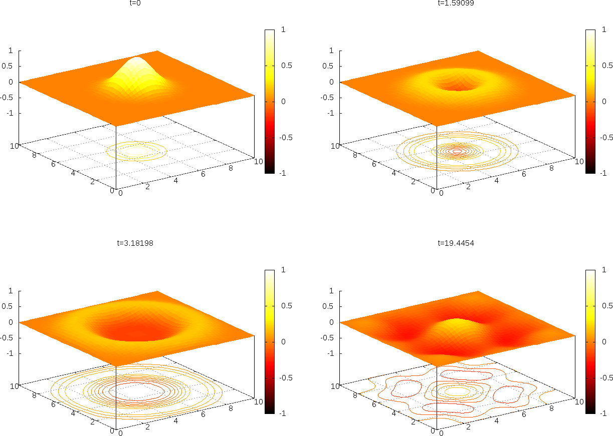
It gives a nice visualization with lifted surface and contours beneath. Figure 31 shows four plots of \( u \).
Figure 31: Snapshots of the surface plotted by Gnuplot.
Video files can be made of the PNG frames:
Terminal> ffmpeg -i tmp_%04d.png -r 25 -vcodec flv movie.flv
Terminal> ffmpeg -i tmp_%04d.png -r 25 -vcodec linx264 movie.mp4
Terminal> ffmpeg -i tmp_%04d.png -r 25 -vcodec libvpx movie.webm
Terminal> ffmpeg -i tmp_%04d.png -r 25 -vcodec libtheora movie.ogg
It is wise to use a high frame rate – a low one will just skip many frames. There may also be considerable quality differences between the different formats.
Mayavi
The best option for doing visualization of 2D and 3D scalar and vector fields in Python programs is Mayavi, which is an interface to the high-quality package VTK in C++. There is good online documentation and also an introduction in Chapter 5 of [6].
To obtain Mayavi on Ubuntu platforms you can write
pip install mayavi --upgrade
For Mac OS X and Windows, we recommend using Anaconda. To obtain Mayavi for Anaconda you can write
conda install mayavi
Mayavi has a MATLAB-like interface called mlab. We can do
import mayavi.mlab as plt
# or
from mayavi import mlab
and have plt (as usual) or mlab
as a kind of MATLAB visualization access inside our program (just
more powerful and with higher visual quality).
The official documentation of the mlab module is provided in two
places, one for the basic functionality
and one for further functionality.
Basic figure
handling
is very similar to the one we know from Matplotlib. Just as for
Matplotlib, all plotting commands you do in mlab will go into the
same figure, until you manually change to a new figure.
Back to our application, the following code for the user action function with plotting in Mayavi is relevant to add.
# Top of the file
try:
    import mayavi.mlab as mlab
except:
    # We don't have mayavi
    pass

def solver(...):
    ...

def gaussian(...):
    ...
    if plot_method == 3:
        from mpl_toolkits.mplot3d import axes3d
        import matplotlib.pyplot as plt
        from matplotlib import cm
        plt.ion()
        fig = plt.figure()
        u_surf = None

    def plot_u(u, x, xv, y, yv, t, n):
        """User action function for plotting."""
        if t[n] == 0:
            time.sleep(2)
        if plot_method == 1:
            # Works well with Gnuplot backend, not with Matplotlib
            st.mesh(x, y, u, title='t=%g' % t[n], zlim=[-1,1],
                    caxis=[-1,1])
        elif plot_method == 2:
            # Works well with Gnuplot backend, not with Matplotlib
            st.surfc(xv, yv, u, title='t=%g' % t[n], zlim=[-1, 1],
                  colorbar=True, colormap=st.hot(), caxis=[-1,1],
                  shading='flat')
        elif plot_method == 3:
            print 'Experimental 3D matplotlib...not recommended'
        elif plot_method == 4:
	    # Mayavi visualization
            mlab.clf()
            extent1 = (0, 20, 0, 20,-2, 2)
            s = mlab.surf(x , y, u,
                          colormap='Blues',
                          warp_scale=5,extent=extent1)
            mlab.axes(s, color=(.7, .7, .7), extent=extent1,
                      ranges=(0, 10, 0, 10, -1, 1),
                      xlabel='', ylabel='', zlabel='',
                      x_axis_visibility=False,
                      z_axis_visibility=False)
            mlab.outline(s, color=(0.7, .7, .7), extent=extent1)
            mlab.text(6, -2.5, '', z=-4, width=0.14)
            mlab.colorbar(object=None, title=None,
                          orientation='horizontal',
                          nb_labels=None, nb_colors=None,
                          label_fmt=None)
            mlab.title('Gaussian t=%g' % t[n])
            mlab.view(142, -72, 50)
            f = mlab.gcf()
            camera = f.scene.camera
            camera.yaw(0)

        if plot_method > 0:
            time.sleep(0) # pause between frames
            if save_plot:
                filename = 'tmp_%04d.png' % n
		if plot_method == 4:
                    mlab.savefig(filename)  # time consuming!
		elif plot_method in (1,2):
                    st.savefig(filename)  # time consuming!
This is a point to get started – visualization is as always a very
time-consuming and experimental discipline. With the PNG files we
can use ffmpeg to create videos.
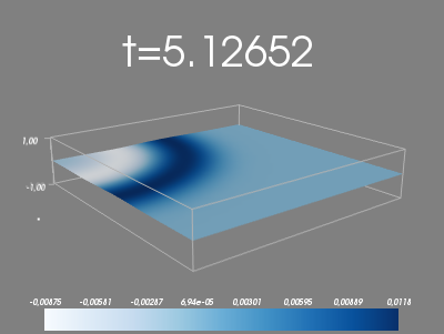
Figure 32: Plot with Mayavi.
Exercises
Exercise 2.16: Check that a solution fulfills the discrete model
Carry out all mathematical details to show that
(2.115) is indeed a solution of the
discrete model for a 2D wave equation with \( u=0 \) on the boundary.
One must check the boundary conditions, the initial conditions,
the general discrete equation at a time level and the special
version of this equation for the first time level.
Filename: check_quadratic_solution.
Project 2.17: Calculus with 2D mesh functions
The goal of this project is to redo Project 2.6: Calculus with 1D mesh functions with 2D mesh functions (\( f_{i,j} \)).
Differentiation.
The differentiation results in a discrete gradient
function, which in the 2D case can be represented by a three-dimensional
array df[d,i,j] where d represents the direction of
the derivative, and i,j is a mesh point in 2D.
Use centered differences for
the derivative at inner points and one-sided forward or backward
differences at the boundary points. Construct unit tests and
write a corresponding test function.
Integration. The integral of a 2D mesh function \( f_{i,j} \) is defined as $$ F_{i,j} = \int_{y_0}^{y_j} \int_{x_0}^{x_i} f(x,y)dxdy,$$ where \( f(x,y) \) is a function that takes on the values of the discrete mesh function \( f_{i,j} \) at the mesh points, but can also be evaluated in between the mesh points. The particular variation between mesh points can be taken as bilinear, but this is not important as we will use a product Trapezoidal rule to approximate the integral over a cell in the mesh and then we only need to evaluate \( f(x,y) \) at the mesh points.
Suppose \( F_{i,j} \) is computed. The calculation of \( F_{i+1,j} \)
is then
$$
\begin{align*}
F_{i+1,j} &= F_{i,j} + \int_{x_i}^{x_{i+1}}\int_{y_0}^{y_j} f(x,y)dydx\\
& \approx \Delta x \half\left(
\int_{y_0}^{y_j} f(x_{i},y)dy
+ \int_{y_0}^{y_j} f(x_{i+1},y)dy\right)
\end{align*}
$$
The integrals in the \( y \) direction can be approximated by a Trapezoidal
rule. A similar idea can be used to compute \( F_{i,j+1} \). Thereafter,
\( F_{i+1,j+1} \) can be computed by adding the integral over the final
corner cell to \( F_{i+1,j} + F_{i,j+1} - F_{i,j} \). Carry out the
details of these computations and implement a function that can
return \( F_{i,j} \) for all mesh indices \( i \) and \( j \). Use the
fact that the Trapezoidal rule is exact for linear functions and
write a test function.
Filename: mesh_calculus_2D.
Exercise 2.18: Implement Neumann conditions in 2D
Modify the wave2D_u0.py program, which solves the 2D wave equation \( u_{tt}=c^2(u_{xx}+u_{yy}) \) with constant wave velocity \( c \) and \( u=0 \) on the boundary, to have Neumann boundary conditions: \( \partial u/\partial n=0 \). Include both scalar code (for debugging and reference) and vectorized code (for speed).
To test the code, use \( u=1.2 \) as solution (\( I(x,y)=1.2 \), \( V=f=0 \), and
\( c \) arbitrary), which should be exactly reproduced with any mesh
as long as the stability criterion is satisfied.
Another test is to use the plug-shaped pulse
in the pulse function from the section Building a general 1D wave equation solver
and the wave1D_dn_vc.py
program. This pulse
is exactly propagated in 1D if \( c\Delta t/\Delta x=1 \). Check
that also the 2D program can propagate this pulse exactly
in \( x \) direction (\( c\Delta t/\Delta x=1 \), \( \Delta y \) arbitrary)
and \( y \) direction (\( c\Delta t/\Delta y=1 \), \( \Delta x \) arbitrary).
Filename: wave2D_dn.
Exercise 2.19: Test the efficiency of compiled loops in 3D
Extend the wave2D_u0.py code and the Cython, Fortran, and C versions to 3D.
Set up an efficiency experiment to determine the relative efficiency of
pure scalar Python code, vectorized code, Cython-compiled loops,
Fortran-compiled loops, and C-compiled loops.
Normalize the CPU time for each mesh by the fastest version.
Filename: wave3D_u0.