Introduction to Scientific Python programming.
Adapted to TKT4140 Numerical Methods
Sep 18, 2017
Table of contents
This is a very quick intro to Python programming
Variables, loops, lists, and arrays
Do you have access to Python?
Mathematical example
A program for evaluating a formula
Assignment statements assign a name to an object
Formatted output with text and numbers
Programming with a while loop
Output of the previous program
Structure of a while loop
Let's take a closer look at the output of our program
Let's examine the program in the Python Online Tutor
Ooops, why is a <= 1.2 when a is 1.2? Round-off errors!
Rule: never a == b for real a and b! Always use a tolerance!
A list collects several objects in a given sequence
Store our table in two lists, one for each column
For loops
Traditional for loop: integer counter over list/array indices
Let's replace our while loop by a for loop
Traversal of multiple lists at the same time with zip
Arrays are computationally efficient lists of numbers
Examples on using arrays
numpy functions creates entire arrays at once
Let's use arrays in our previous program
Standard mathematical functions are found in the math module
Use the numpy module for standard mathematical functions applied to arrays
Array assignment gives view (no copy!) of array data
Copying array data requires special action via the copy method
Construction of tridiagonal and sparse matrices
Example on constructing a tridiagonal matrix using spdiags
Example on constructing a tridiagonal matrix using diags
Example on solving a tridiagonal system
Plotting
Plotting of multiple curves
Functions and branching
Functions
Functions can have multiple arguments
Keyword arguments are arguments with default values
Vectorization speeds up the code
Python functions written for scalars normally work for arrays too!
Python functions can return multiple values
A more general mathematical formula (part I)
A more general mathematical formula (part II)
Basic if-else tests
Multi-branch if tests
Implementation of a piecewisely defined function with if
Python functions containing if will not accept array arguments
Remedy 1: Call the function with scalar arguments
Remedy 2: Vectorize the if test with where
Remedy 3: Vectorize the if test with array indexing
Files
File reading
Code for reading files with lines variable = value
Splitting lines into words is a frequent operation
The magic eval function
Implementing a calculator in Python
Modern Python often applies the with statement for file handling
File writing
Simplified writing of tabular data to file via numpy.savetxt
Simplified reading of tabular data from file via numpy.loadtxt
Classes
A very simple class
How can we use this class?
The self argument is a difficult thing for newcomers...
A class for representing a mathematical function
The class code
Class implementation of \( f(x,y,z; p_1,p_2,\ldots,p_n) \)
This is a very quick intro to Python programming
- variables for numbers, lists, and arrays
- while loops and for loops
- functions
- if tests
- plotting
- files
- classes
Variables, loops, lists, and arrays

Do you have access to Python?
Many methods:
- Mac and Windows: Anaconda
- Ubuntu:
sudo apt-get install - Web browser (Wakari or SageMathCloud)
Mathematical example
Most examples will involve this formula: $$ \begin{equation} \label{basics:seq} s = v_0t + \frac{1}{2}at^2 \end{equation} $$ We may view \( s \) as a function of \( t \): \( s(t) \), and also include the parameters in the notation: \( s(t;v_0,a) \).
A program for evaluating a formula
t = 0.5
v0 = 2
a = 0.2
s = v0*t + 0.5*a*t**2
print s
Terminal> python distance.py
1.025
Assignment statements assign a name to an object
t = 0.5                   # real number makes float object
v0 = 2                    # integer makes int object
a = 0.2                   # float object
s = v0*t + 0.5*a*t**2     # float object
Rule:
- evaluate right-hand side; it results in an object
- left-hand side is a name for that object
Formatted output with text and numbers
- Task: write out text with a number (3 decimals):
s=1.025 - Method: printf syntax
print 's=%g' % s       # g: compact notation
print 's=%.2f' % s     # f: decimal notation, .2f: 2 decimals
Modern alternative: format string syntax
print 's={s:.2f}'.format(s=s)
Programming with a while loop
- Task: write out a table of \( t \) and \( s(t) \) values (two columns), for \( t\in [0,2] \) in steps of 0.1
- Method: while loop
v0 = 2
a = 0.2
dt = 0.1  # Increment
t = 0     # Start value
while t <= 2:
    s = v0*t + 0.5*a*t**2
    print t, s
    t = t + dt
Output of the previous program
Terminal> python while.py
0 0.0
0.1 0.201
0.2 0.404
0.3 0.609
0.4 0.816
0.5 1.025
0.6 1.236
0.7 1.449
0.8 1.664
0.9 1.881
1.0 2.1
1.1 2.321
1.2 2.544
1.3 2.769
1.4 2.996
1.5 3.225
1.6 3.456
1.7 3.689
1.8 3.924
1.9 4.161
Structure of a while loop
while condition:
    <intented statement>
    <intented statement>
    <intented statement>
Note:
- the colon in the first line
- all statements in the loop must be indented
(no braces as in C, C++, Java, ...) -
conditionis a boolean expression (e.g.,t <= 2)
Let's take a closer look at the output of our program
Terminal> python while.py
0 0.0
0.1 0.201
0.2 0.404
...
1.8 3.924
1.9 4.161
The last line contains 1.9, but the while loop should run also when
\( t=2 \) since the test is t <= 2. Why is this test False?
Let's examine the program in the Python Online Tutor
Python Online Tutor: step through the program and examine variables (view in Chrome)
Ooops, why is a <= 1.2 when a is 1.2? Round-off errors!
da makes a = 1.2000000000000002
Rule: never a == b for real a and b! Always use a tolerance!
a = 1.2
b = 0.4 + 0.4 + 0.4
boolean_condition1 = a == b              # may be False

# This is the way to do it
tol = 1E-14
boolean_condition2 = abs(a - b) < tol    # True
A list collects several objects in a given sequence
A list of numbers:
L = [-1, 1, 8.0]
A list can contain any type of objects, e.g.,
L = ['mydata.txt', 3.14, 10] # string, float, int
Some basic list operations:
>>> L = ['mydata.txt', 3.14, 10]
>>> print L[0]    # print first element (index 0)
mydata.txt
>>> print L[1]    # print second element (index 1)
3.14
>>> del L[0]      # delete the first element
>>> print L
[3.14, 10]
>>> print len(L)  # length of L
2
>>> L.append(-1)  # add -1 at the end of the list
>>> print L
[3.14, 10, -1]
Store our table in two lists, one for each column
v0 = 2
a = 0.2
dt = 0.1  # Increment
t = 0
t_values = []
s_values = []
while t <= 2:
    s = v0*t + 0.5*a*t**2
    t_values.append(t)
    s_values.append(s)
    t = t + dt
print s_values  # Just take a look at a created list

# Print a nicely formatted table
i = 0
while i <= len(t_values)-1:
    print '%.2f  %.4f' % (t_values[i], s_values[i])
    i += 1   # Same as i = i + 1
For loops
A for loop is used for visiting elements in a list, one by one:
>>> L = [1, 4, 8, 9]
>>> for e in L:
...     print e
...
1
4
8
9
Demo in the Python Online Tutor:
Traditional for loop: integer counter over list/array indices
somelist = ['file1.dat', 22, -1.5]

for i in range(len(somelist)):
    # access list element through index
    print somelist[i]
Note:
-
rangereturns a list of integers -
range(a, b, s)returns the integersa, a+s, a+2*s, ...up to but not including (!!)b -
range(b)impliesa=0ands=1 -
range(len(somelist))returns[0, 1, 2]
Let's replace our while loop by a for loop
v0 = 2
a = 0.2
dt = 0.1  # Increment
t_values = []
s_values = []
n = int(round(2/dt)) + 1  # No of t values
for i in range(n):
    t = i*dt
    s = v0*t + 0.5*a*t**2
    t_values.append(t)
    s_values.append(s)
print s_values  # Just take a look at a created list

# Make nicely formatted table
for t, s in zip(t_values, s_values):
    print '%.2f  %.4f' % (t, s)

# Alternative implementation
for i in range(len(t_values)):
    print '%.2f  %.4f' % (t_values[i], s_values[i])
Traversal of multiple lists at the same time with zip
for e1, e2, e3, ... in zip(list1, list2, list3, ...):
Alternative: loop over a common index for the lists
for i in range(len(list1)):
    e1 = list1[i]
    e2 = list2[i]
    e3 = list3[i]
    ...
Arrays are computationally efficient lists of numbers
- Lists collect a set of objects in a single variable
- Lists are very flexible (can grow, can contain "anything")
- Array: computationally efficient and convenient list
- Arrays must have fixed length and can only contain numbers of the same type (integers, real numbers, complex numbers)
- Arrays require the
numpymodule
Examples on using arrays
>>> import numpy
>>> L = [1, 4, 10.0]    # List of numbers
>>> a = numpy.array(L)  # Convert to array
>>> print a
[  1.   4.  10.]
>>> print a[1]          # Access element through indexing
4.0
>>> print a[0:2]        # Extract slice (index 2 not included!)
[  1.   4.]
>>> print a.dtype       # Data type of an element
float64
>>> b = 2*a + 1         # Can do arithmetics on arrays
>>> print b
[  3.   9.  21.]
numpy functions creates entire arrays at once
Apply \( \ln \) to all elements in array a:
>>> c = numpy.log(a)
>>> print c
[ 0.          1.38629436  2.30258509]
Create \( n+1 \) uniformly distributed coordinates in \( [a,b] \):
t = numpy.linspace(a, b, n+1)
Create array of length \( n \) filled with zeros:
t = numpy.zeros(n)
s = numpy.zeros_like(t)  # zeros with t's size and data type
Let's use arrays in our previous program
import numpy
v0 = 2
a = 0.2
dt = 0.1  # Increment
n = int(round(2/dt)) + 1  # No of t values

t_values = numpy.linspace(0, 2, n+1)
s_values = v0*t + 0.5*a*t**2

# Make nicely formatted table
for t, s in zip(t_values, s_values):
    print '%.2f  %.4f' % (t, s)
Note: no explicit loop for computing s_values!
Standard mathematical functions are found in the math module
>>> import math
>>> print math.sin(math.pi)
1.2246467991473532e-16         # Note: only approximate value
Get rid of the math prefix:
from math import sin, pi
print sin(pi)

# Or import everything from math
from math import *
print sin(pi), log(e), tanh(0.5)
Use the numpy module for standard mathematical functions applied to arrays
Matlab users can do
from numpy import *
x = linspace(0, 1, 101)
y = exp(-x)*sin(pi*x)
The Python community likes
import numpy as np
x = np.linspace(0, 1, 101)
y = np.exp(-x)*np.sin(np.pi*x)
Our convention: use np prefix, but not in formulas involving
math functions
import numpy as np
x = np.linspace(0, 1, 101)

from numpy import sin, exp, pi
y = exp(-x)*sin(pi*x)
Array assignment gives view (no copy!) of array data
Consider array assignment b=a:
a = np.linspace(1, 5, 5)
b = a
Here, b is a just view or a pointer to the data of a - no copying of
data!
See the following example how changes in b inflict changes in a
>>> a
array([ 1.,  2.,  3.,  4.,  5.])
>>> b[0] = 5                          # changes a[0] to 5
>>> a
array([ 5.,  2.,  3.,  4.,  5.])
>>> a[1] = 9                          # changes b[1] to 9
>>> b
array([ 5.,  9.,  3.,  4.,  5.])
Copying array data requires special action via the copy method
>>> c = a.copy()       # copy all elements to new array c
>>> c[0] = 6           # a is not changed
>>> a
array([ 1.,  2.,  3.,  4.,  5.])
>>> c
array([ 6.,  2.,  3.,  4.,  5.])
>>> b
array([ 5.,  2.,  3.,  4.,  5.])
Note: b has still the values from the previous example
Construction of tridiagonal and sparse matrices
- SciPy offers a sparse matrix package scipy.sparse
- The
spdiagsfunction may be used to construct a sparse matrix from diagonals - Note that all the diagonals must have the same length as the dimension of their sparse matrix - consequently some elements of the diagonals are not used
- The first \( k \) elements are not used of the \( k \) super-diagonal
- The last \( k \) elements are not used of the \( -k \) sub-diagonal
Example on constructing a tridiagonal matrix using spdiags
>>> import numpy as np
>>> N = 6
>>> diagonals = np.zeros((3, N))   # 3 diagonals
diagonals[0,:] = np.linspace(-1, -N, N)
diagonals[1,:] = -2
diagonals[2,:] = np.linspace(1, N, N)
>>> import scipy.sparse
>>> A = scipy.sparse.spdiags(diagonals, [-1,0,1], N, N, format='csc')
>>> A.toarray()    # look at corresponding dense matrix
[[-2.  2.  0.  0.  0.  0.]
 [-1. -2.  3.  0.  0.  0.]
 [ 0. -2. -2.  4.  0.  0.]
 [ 0.  0. -3. -2.  5.  0.]
 [ 0.  0.  0. -4. -2.  6.]
 [ 0.  0.  0.  0. -5. -2.]]
Example on constructing a tridiagonal matrix using diags
An alternative function that may be used to construct sparse matrices is thediags function. It differs from spdiags
in the way it handles of diagonals.
- All diagonals need to be given with their correct lengths (i.e. super- and sub-diagonals are shorter than the main diagonal)
- It also supports scalar broadcasting
>>> diagonals = [-np.linspace(1, N, N)[0:-1], -2*np.ones(N), np.linspace(1, N, N)[1:]]   # 3 diagonals
>>> A = scipy.sparse.diags(diagonals, [-1,0,1], format='csc')
>>> A.toarray()    # look at corresponding dense matrix
[[-2.  2.  0.  0.  0.  0.]
 [-1. -2.  3.  0.  0.  0.]
 [ 0. -2. -2.  4.  0.  0.]
 [ 0.  0. -3. -2.  5.  0.]
 [ 0.  0.  0. -4. -2.  6.]
 [ 0.  0.  0.  0. -5. -2.]]
Here's an example using scalar broadcasting (need to specify shape):
>>> B = scipy.sparse.diags([1, 2, 3], [-2, 0, 1], shape=(6, 6), format='csc')
>>> B.toarray()    # look at corresponding dense matrix
[[ 2.  3.  0.  0.  0.  0.]
 [ 0.  2.  3.  0.  0.  0.]
 [ 1.  0.  2.  3.  0.  0.]
 [ 0.  1.  0.  2.  3.  0.]
 [ 0.  0.  1.  0.  2.  3.]
 [ 0.  0.  0.  1.  0.  2.]]
Example on solving a tridiagonal system
We can solve \( Ax=b \) with tridiagonal matrix \( A \): choose some \( x \), compute \( b=Ax \) (sparse/tridiagonal matrix product!), solve \( Ax=b \), and check that \( x \) is the desired solution:
>>> x = np.linspace(-1, 1, N)  # choose solution
>>> b = A.dot(x)               # sparse matrix vector product
>>> import scipy.sparse.linalg
>>> x = scipy.sparse.linalg.spsolve(A, b)
>>> print x
[-1.  -0.6 -0.2  0.2  0.6  1. ]
Check against dense matrix computations:
>>> A_d = A.toarray()            # corresponding dense matrix
>>> b = np.dot(A_d, x)           # standard matrix vector product
>>> x = np.linalg.solve(A_d, b)  # standard Ax=b algorithm
>>> print x
[-1.  -0.6 -0.2  0.2  0.6  1. ]
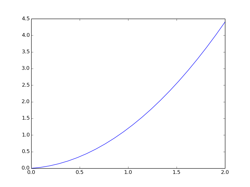
Plotting
Plotting is done with matplotlib:
import numpy as np
import matplotlib.pyplot as plt

v0 = 0.2
a = 2
n = 21  # No of t values for plotting

t = np.linspace(0, 2, n+1)
s = v0*t + 0.5*a*t**2

plt.plot(t, s)
plt.savefig('myplot.png')
plt.show()
The plotfile myplot.png looks like
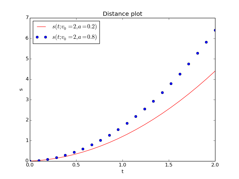
Plotting of multiple curves
import numpy as np
import matplotlib.pyplot as plt

v0 = 0.2
n = 21  # No of t values for plotting

t = np.linspace(0, 2, n+1)
a = 2
s0 = v0*t + 0.5*a*t**2
a = 3
s1 = v0*t + 0.5*a*t**2

plt.plot(t, s0, 'r-',  # Plot s0 curve with red line
         t, s1, 'bo')  # Plot s1 curve with blue circles
plt.xlabel('t')
plt.ylabel('s')
plt.title('Distance plot')
plt.legend(['$s(t; v_0=2, a=0.2)$', '$s(t; v_0=2, a=0.8)$'],
           loc='upper left')
plt.savefig('myplot.png')
plt.show()
Functions and branching

Functions
- \( s(t)=v_0t + \frac{1}{2}at^2 \) is a mathematical function
- Can implement \( s(t) \) as a Python function
s(t)
def s(t):
    return v0*t + 0.5*a*t**2

v0 = 0.2
a = 4
value = s(3)   # Call the function
Note:
- functions start with the keyword
def - statements belonging to the function must be indented
- function input is represented by arguments (separated by comma if more than one)
- function output is returned to the calling code
-
v0andaare global variables, which must be initialized befores(t)is called
Functions can have multiple arguments
v0 and a as function arguments instead of global variables:
def s(t, v0, a):
    return v0*t + 0.5*a*t**2

value = s(3, 0.2, 4)   # Call the function

# More readable call
value = s(t=3, v0=0.2, a=4)
Keyword arguments are arguments with default values
def s(t, v0=1, a=1):
    return v0*t + 0.5*a*t**2

value = s(3, 0.2, 4)         # specify new v0 and a
value = s(3)                 # rely on v0=1 and a=1
value = s(3, a=2)            # rely on v0=1
value = s(3, v0=2)           # rely on a=1
value = s(t=3, v0=2, a=2)    # specify everything
value = s(a=2, t=3, v0=2)    # any sequence allowed
- Arguments without the argument name are called positional arguments
- Positional arguments must always be listed before the keyword arguments in the function and in any call
- The sequence of the keyword arguments can be arbitrary
Vectorization speeds up the code
Scalar code (work with one number at a time):
def s(t, v0, a):
    return v0*t + 0.5*a*t**2

for i in range(len(t)):
    s_values[i] = s(t_values[i], v0, a)
Vectorized code: apply s to the entire array
s_values = s(t_values, v0, a)
How can this work?
- Expression: v0*t + 0.5*a*t**2 with array
t -
r1 = v0*t(scalar times array) -
r2 = t**2(square each element) -
r3 = 0.5*a*r2(scalar times array) -
r1 + r3(add each element)
Python functions written for scalars normally work for arrays too!
True if computations involve arithmetic operations and math functions:
from math import exp, sin

def f(x):
    return 2*x + x**2*exp(-x)*sin(x)

v = f(4)  # f(x) works with scalar x

# Redefine exp and sin with their vectorized versions
from numpy import exp, sin, linspace
x = linspace(0, 4, 100001)
v = f(x)  # f(x) works with array x
Python functions can return multiple values
Return \( s(t)=v_0t+\frac{1}{2}at^2 \) and \( s'(t)=v_0 + at \):
def movement(t, v0, a):
    s = v0*t + 0.5*a*t**2
    v = v0 + a*t
    return s, v

s_value, v_value = movement(t=0.2, v0=2, a=4)
return s, v means that we return a tuple (\( \approx \) list):
>>> def f(x):
...     return x+1, x+2, x+3
...
>>> r = f(3)     # Store all three return values in one object r
>>> print r
(4, 5, 6)
>>> type(r)      # What type of object is r?
<type 'tuple'>
>>> print r[1]
5
Tuples are constant lists (cannot be changed)
A more general mathematical formula (part I)
Equations from basic kinematics: $$ \begin{align*} v = \frac{ds}{dt},\quad s(0)=s_0\\ a = \frac{dv}{dt},\quad v(0)=v_0 \end{align*} $$
Integrate to find \( v(t) \): $$ \int_0^t a(t)dt = \int_0^t \frac{dv}{dt} dt$$ which gives $$ v(t) = v_0 + \int_0^t a(t)dt $$
A more general mathematical formula (part II)
Integrate again over \( [0,t] \) to find \( s(t) \): $$ s(t) = s_0 + v_0t + \int_0^t\left( \int_0^t a(t)dt \right) dt$$
Example: \( a(t)=a_0 \) for \( t\in[0,t_1] \), then \( a(t)=0 \) for \( t>t_1 \): $$ s(t) = \left\lbrace\begin{array}{ll} s_0 + v_0 t + \frac{1}{2}a_0 t^2,& t\leq t_1\\ s_0 + v_0t_1 + \frac{1}{2}a_0 t_1^2 + a_0t_1(t-t_1),& t> t_1 \end{array}\right. $$
Need if test to implement this!
Basic if-else tests
An if test has the structure
if condition:
    <statements when condition is True>
else:
    <statements when condition is False>
Here,
-
conditionis a boolean expression with valueTrueorFalse.
if t <= t1:
    s = v0*t + 0.5*a0*t**2
else:
    s = v0*t + 0.5*a0*t1**2 + a0*t1*(t-t1)
Multi-branch if tests
if condition1:
    <statements when condition1 is True>
elif condition2:
    <statements when condition1 is False and condition2 is True>
elif condition3:
    <statements when condition1 and conditon 2 are False
     and condition3 is True>
else:
    <statements when condition1/2/3 all are False>
Just if, no else:
if condition:
    <statements when condition is True>
Implementation of a piecewisely defined function with if
A Python function implementing the mathematical function $$ s(t) = \left\lbrace\begin{array}{ll} s_0 + v_0 t + \frac{1}{2}a_0 t^2,& t\leq t_1\\ s_0 + v_0t_1 + \frac{1}{2}a_0 t_1^2 + a_0t_1(t-t_1),& t> t_1 \end{array}\right. $$
reads
def s_func(t, v0, a0, t1):
    if t <= t1:
        s = v0*t + 0.5*a0*t**2
    else:
        s = v0*t + 0.5*a0*t1**2 + a0*t1*(t-t1)
    return s
Python functions containing if will not accept array arguments
>>> def f(x): return x if x < 1 else 2*x
...
>>> import numpy as np
>>> x = np.linspace(0, 2, 5)
>>> f(x)
Traceback (most recent call last):
...
ValueError: The truth value of an array with more than one
element is ambiguous. Use a.any() or a.all()
Problem: x < 1 evaluates to a boolean array, not just a boolean
Remedy 1: Call the function with scalar arguments
n = 201  # No of t values for plotting
t1 = 1.5

t = np.linspace(0, 2, n+1)
s = np.zeros(n+1)
for i in range(len(t)):
    s[i] = s_func(t=t[i], v0=0.2, a0=20, t1=t1)
Can now easily plot:
plt.plot(t, s, 'b-')
plt.plot([t1, t1], [0, s_func(t=t1, v0=0.2, a0=20, t1=t1)], 'r--')
plt.xlabel('t')
plt.ylabel('s')
plt.savefig('myplot.png')
plt.show()
Remedy 2: Vectorize the if test with where
Functions with if tests require a complete rewrite to work with arrays.
s = np.where(condition, s1, s2)
Explanation:
-
condition: array of boolean values -
s[i] = s1[i]ifcondition[i]isTrue -
s[i] = s2[i]ifcondition[i]isFalse
s = np.where(t <= t1,
             v0*t + 0.5*a0*t**2,
             v0*t + 0.5*a0*t1**2 + a0*t1*(t-t1))
Note that t <= t1 with array t and scalar t1 results in a boolean
array b where b[i] = t[i] <= t1.
Remedy 3: Vectorize the if test with array indexing
- Let
bbe a boolean array (e.g.,b = t <= t1) -
s[b]selects all elementss[i]whereb[i]isTrue - Can assign some array expression
exprof lengthlen(s[b])tos[b]:s[b] = (expr)[b]
b as t <= t1 and t > t1:
s = np.zeros_like(t)  # Make s as zeros, same size & type as t
s[t <= t1] = (v0*t + 0.5*a0*t**2)[t <= t1]
s[t > t1]  = (v0*t + 0.5*a0*t1**2 + a0*t1*(t-t1))[t > t1]
Files

File reading
Put input data in a text file:
v0 = 2
a = 0.2
dt = 0.1
interval = [0, 2]
v0, a, dt, and interval?
Code for reading files with lines variable = value
infile = open('.input.dat', 'r')
for line in infile:
    # Typical line: variable = value
    variable, value = line.split('=')
    variable = variable.strip()  # remove leading/traling blanks
    if variable == 'v0':
        v0 = float(value)
    elif variable == 'a':
        a = float(value)
    elif variable == 'dt':
        dt = float(value)
    elif variable == 'interval':
        interval = eval(value)
infile.close()
Splitting lines into words is a frequent operation
>>> line = 'v0 = 5.3'
>>> variable, value = line.split('=')
>>> variable
'v0 '
>>> value
' 5.3'
>>> variable.strip()  # strip away blanks
'v0'
Note: must convert value to float before we can compute with
the value!
The magic eval function
eval(s) executes a string s as a Python expression and creates the
corresponding Python object
>>> obj1 = eval('1+2')   # Same as obj1 = 1+2
>>> obj1, type(obj1)
(3, <type 'int'>)
>>> obj2 = eval('[-1, 8, 10, 11]')
>>> obj2, type(obj2)
([-1, 8, 10, 11], <type 'list'>)
>>> from math import sin, pi
>>> x = 1
>>> obj3 = eval('sin(pi*x)')
>>> obj3, type(obj3)
(1.2246467991473532e-16, <type 'float'>)
Why is this so great? We can read formulas, lists, expressions as
text from file and with eval turn them into live Python objects!
Implementing a calculator in Python
Demo:
Terminal> python calc.py "1 + 0.5*2"
2.0
Terminal> python calc.py "sin(pi*2.5) + exp(-4)"
1.0183156388887342
Just 5 lines of code:
import sys
command_line_expression = sys.argv[1]
from math import *   # Define sin, cos, exp, pi, etc.
result = eval(command_line_expression)
print result
Modern Python often applies the with statement for file handling
with open('.input.dat', 'r') as infile:
    for line in infile:
        ...
No need to close the file when using with
File writing
- We have \( t \) and \( s(t) \) values in two lists,
t_valuesands_values - Task: write these lists as a nicely formatted table in a file
outfile = open('table1.dat', 'w')
outfile.write('# t    s(t)\n')  # write table header
for t, s in zip(t_values, s_values):
    outfile.write('%.2f  %.4f\n' % (t, s))
Simplified writing of tabular data to file via numpy.savetxt
import numpy as np
# Make two-dimensional array of [t, s(t)] values in each row
data = np.array([t_values, s_values]).transpose()

# Write data array to file in table format
np.savetxt('table2.dat', data, fmt=['%.2f', '%.4f'],
           header='t   s(t)', comments='# ')
table2.dat:
# t   s(t)
0.00 0.0000
0.10 0.2010
0.20 0.4040
0.30 0.6090
0.40 0.8160
0.50 1.0250
0.60 1.2360
...
1.90 4.1610
2.00 4.4000
Simplified reading of tabular data from file via numpy.loadtxt
data = np.loadtxt('table2.dat', comments='#')
Note:
- Lines beginning with the comment character
#are skipped in the reading -
datais a two-dimensional array:data[i,0]holds the \( t \) value anddata[i,1]the \( s(t) \) value in thei-th row
Classes
- All objects in Python are made from a class
- You don't need to know about classes to use Python
- But class programming is powerful
- Class = functions + variables packed together
- A class is a logical unit in a program
- A large program as a combination of appropriate units
A very simple class
- One variable:
a - One function:
dumpfor printinga
class Trivial:
    def __init__(self, a):
        self.a = a

    def dump(self):
        print self.a
Class terminology: Functions are called methods and variables are called attributes.
How can we use this class?
First, make an instance (object) of the class:
t = Trivial(a=4)
t.dump()
Note:
- The syntax
Trivial(a=4)actually meansTrivial.__init__(t, 4) -
selfis an argument in__init__anddump, but not used in the calls -
__init__is called constructor and is used to construct an object (instance) if the class -
t.dump()actually meansTrivial.dump(t)(selfist)
The self argument is a difficult thing for newcomers...
It takes time and experience to understand the self argument in
class methods!
-
selfmust always be the first argument -
selfis never used in calls -
selfis used to access attributes and methods inside methods
self.
self is confusing in the beginning, but later it greatly helps
the understanding of how classes work!
A class for representing a mathematical function
Function with one independent variable \( t \) and two parameters \( v_0 \) and \( a \): $$ s(t; v_0, a) = v_0t + \frac{1}{2}at^2$$
Class representation of this function:
-
v0andaare variables (data) - A method to evaluate \( s(t) \), but just as a function of
t
s = Distance(v0=2, a=0.5)  # create instance
v = s(t=0.2)               # compute formula
The class code
class Distance:
    def __init__(self, v0, a):
        self.v0 = v0
        self.a = a

    def __call__(self, t):
        v0, a = self.v0, self.a  # make local variables
        return v0*t + 0.5*a*t**2

s = Distance(v0=2, a=0.5)  # create instance
v = s(t=0.2)               # actually s.__call__(t=0.2)
Class implementation of \( f(x,y,z; p_1,p_2,\ldots,p_n) \)
- The \( n \) parameters \( p_1,p_2,\ldots,p_n \) are attributes
-
__call__(self, x, y, z)is used to compute \( f(x, y, z) \)
class F:
    def __init__(self, p1, p2, ...):
        self.p1 = p1
        self.p2 = p2
        ...

    def __call__(self, x, y, z):
        # return formula involving x, y, z and self.p1, self.p2 ...

f = F(p1=..., p2=..., ...)   # create instance with parameters
print f(1, 4, -1)            # evaluate f(x,y,z) function