Exercises

Exercise 1: Program a formula

a) Make a simplest possible Python program that calculates and prints the value of the formula $$y = 6x^2 + 3x + 2,\] for $x=2$.$$

Solution.

x = 2
y = 6*x**2 + 3*x + 2
print(y)

b) Make a Python function that takes $x$ as argument and returns $y$. Call the function for $x=2$ and print the answer.

Solution.

def f(x):
    return 6*x**2 + 3*x + 2

y = f(2)
print(y)

Exercise 2: Combine text and numbers in output

Let $y=x^2$. Make a program that writes the text

y(2.550)=6.502

if $x=2.55$. The values of $x$ and $y$ should be written with three decimals. Run the program for $x=\pi$ too (the value if $\pi$ is available as the variable pi in the math module).

Solution.

x = 2.55
y = x**2
print('y(%.3f)=%.3f' % (x, y))

from math import pi
x = pi
y = x**2
print('y(%.3f)=%.3f' % (x, y))

Exercise 3: Program a while loop

Define a sequence of numbers, $$x_n = n^2 + 1,$$ for integers $n=0,1,2,\ldots,N$. Write a program that prints out $x_n$ for $n=0,1,\ldots,20$ using a while loop.

Solution.

n = 0
while n <= 20:
    x_n = n**2 + 1
    print('x%d=%d' % (n, x_n))
    n = n + 1

Exercise 4: Create a list with a while loop

Store all the $x_n$ values computed in Exercise 3: Program a while loop in a list (using a while loop). Print the entire list (as one object).

Solution.

n = 0
x = []  # the x_n values
while n <= 20:
    x.append(n**2 + 1)
    n = n + 1
print(x)

Exercise 5: Program a for loop

Do Exercise 4: Create a list with a while loop, but use a for loop.

Solution.

x = []
for n in range(21):
    x.append(n**2 + 1)
print(x)

x = [n**2 + 1 for n in range(21)]
print(x)

Exercise 6: Write a Python function

Write a function x(n) for computing an element in the sequence $x_n=n^2+1$. Call the function for $n=4$ and write out the result.

Solution.

def x(n):
    return n^2 + 1

print(x(4))

Exercise 7: Return three values from a Python function

Write a Python function that evaluates the mathematical functions $f(x)=\cos(2x)$, $f'(x)=-2\sin(2x)$, and $f''(x)=-4\cos(2x)$. Return these three values. Write out the results of these values for $x=\pi$.

Solution.

from math import sin, cos, pi

def deriv2(x):
    return cos(2*x), -2*sin(2*x), -4*cos(2*x)

f, df, d2f = deriv2(x=pi)
print(f, df, d2f)

Terminal> python deriv2.py
1.0 4.89858719659e-16 -4.0

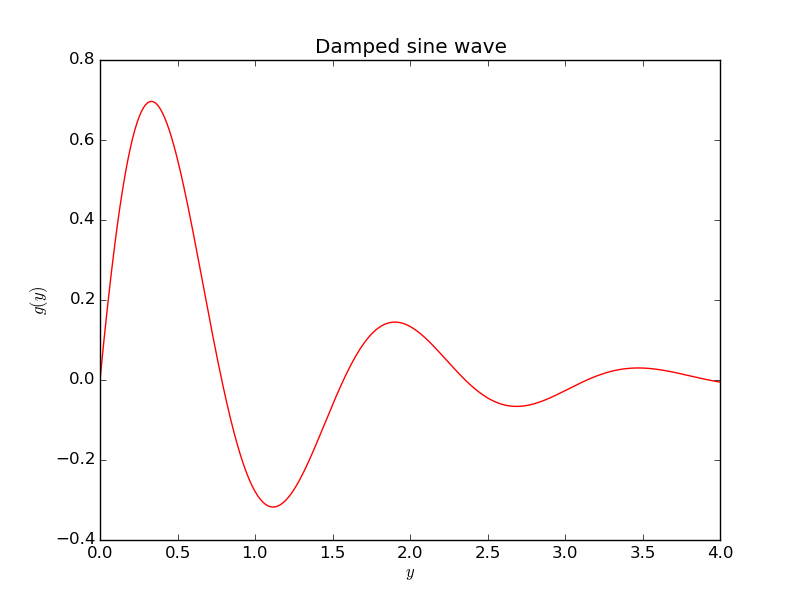
Exercise 8: Plot a function

Make a program that plots the function $g(y)=e^{-y}\sin (4y)$ for $y\in [0,4]$ using a red solid line. Use 500 intervals for evaluating points in $[0,4]$. Store all coordinates and values in arrays. Set labels on the axis and use a title "Damped sine wave".

Solution.

import numpy as np
import matplotlib.pyplot as plt
from numpy import exp, sin  # avoid np. prefix in g(y) formula

def g(y):
    return exp(-y)*sin(4*y)

y = np.linspace(0, 4, 501)
values = g(y)
plt.figure()
plt.plot(y, values, 'r-')
plt.xlabel('$y$'); plt.ylabel('$g(y)$')
plt.title('Damped sine wave')
plt.savefig('tmp.png'); plt.savefig('tmp.pdf')
plt.show()

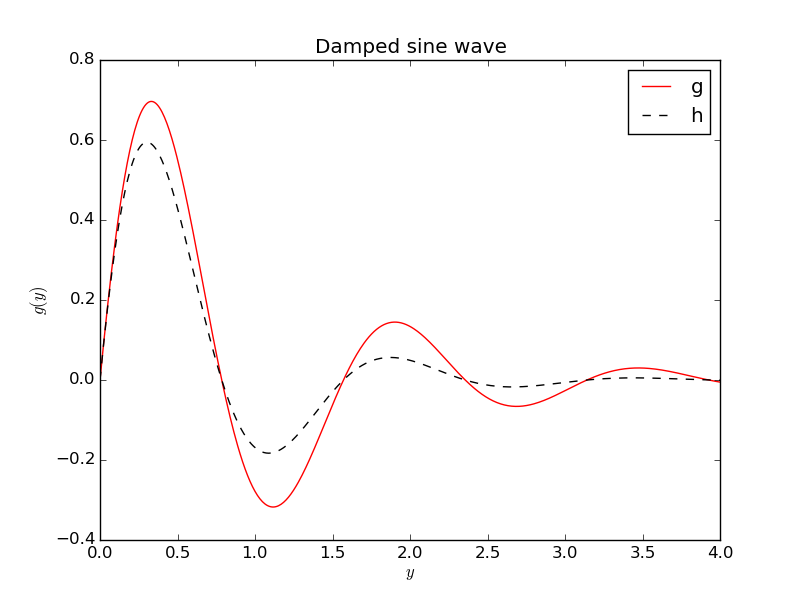
Exercise 9: Plot two functions

As Exercise 9: Plot two functions, but add a black dashed curve for the function $h(y)=e^{-\frac{3}{2}y}\sin (4y)$. Include a legend for each curve (with names g and h).

Solution.

import numpy as np
import matplotlib.pyplot as plt
from numpy import exp, sin  # avoid np. prefix in g(y) and h(y)

def g(y):
    return exp(-y)*sin(4*y)

def h(y):
    return exp(-(3./2)*y)*sin(4*y)

y = np.linspace(0, 4, 501)
plt.figure()
plt.plot(y, g(y), 'r-', y, h(y), 'k--')
plt.xlabel('$y$'); plt.ylabel('$g(y)$')
plt.title('Damped sine wave')
plt.legend(['g', 'h'])
plt.savefig('tmp.png'); plt.savefig('tmp.pdf')
plt.show()

Exercise 10: Measure the efficiency of vectorization

IPython an enhanced interactive shell for doing computing with Python. IPython has some user-friendly functionality for quick testing of the efficiency of different Python constructions. Start IPython by writing ipython in a terminal window. The interactive session below demonstrates how we can use the timer feature %timeit to measure the CPU time required by computing $\sin (x)$, where $x$ is an array of 1M elements, using scalar computing with a loop (function sin_func) and vectorized computing using the sin function from numpy.

In [1]: import numpy as np

In [2]: n = 1000000

In [3]: x = np.linspace(0, 1, n+1)

In [4]: def sin_func(x):
   ...:     r = np.zeros_like(x)  # result
   ...:     for i in range(len(x)):
   ...:         r[i] = np.sin(x[i])
   ...:     return r
   ...:

In [5]: %timeit y = sin_func(x)
1 loops, best of 3: 2.68 s per loop

In [6]: %timeit y = np.sin(x)
10 loops, best of 3: 40.1 ms per loop

Here, %timeit ran our function once, but the vectorized function 10 times. The most relevant CPU times measured are listed, and we realize that the vectorized code is $2.68/(40.1/1000)\approx 67$ times faster than the loop-based scalar code.

Use the recipe above to investigate the speed up of the vectorized computation of the $s(t)$ function in the section Functions.

• «
• 1
• 2
• 3
• 4
• 5
• 6