Newton's method
Newton's method, also known as Newton-Raphson's method, is a very famous and widely used method for solving nonlinear algebraic equations. Compared to the other methods we will consider, it is generally the fastest one (usually by far). It does not guarantee that an existing solution will be found, however.
A fundamental idea of numerical methods for nonlinear equations is to construct a series of linear equations (since we know how to solve linear equations) and hope that the solutions of these linear equations bring us closer and closer to the solution of the nonlinear equation. The idea will be clearer when we present Newton's method and the secant method.
Deriving and implementing Newton's method
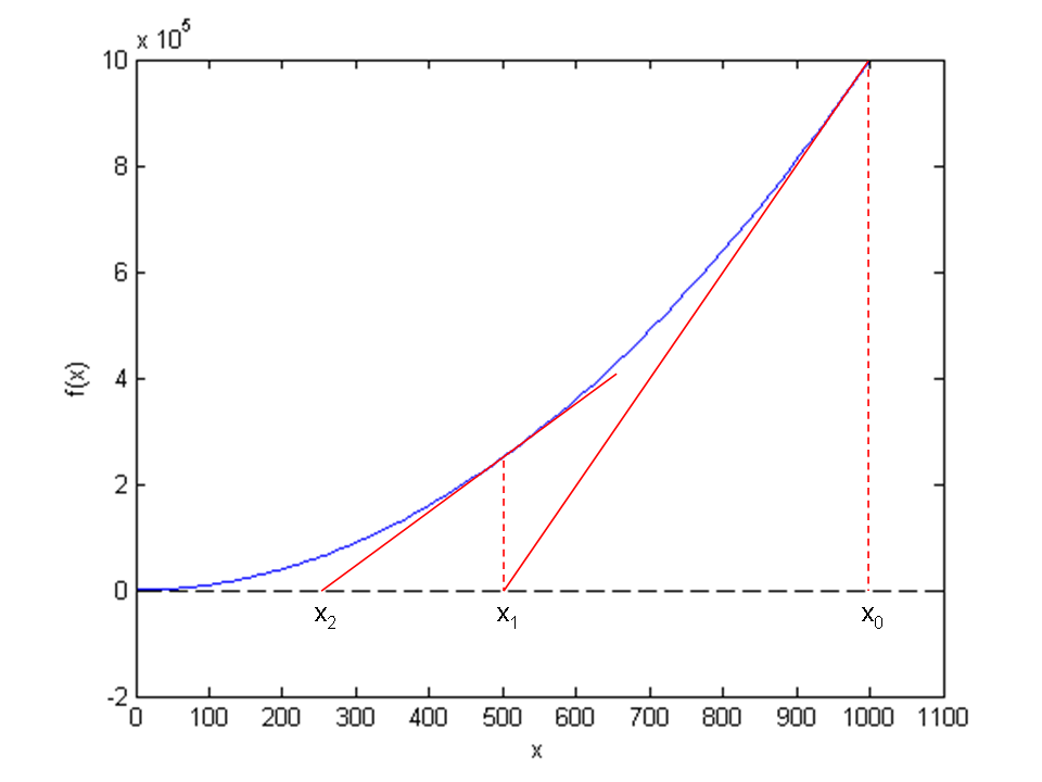
Figure 62 shows the \( f(x) \) function in our model equation \( x^2-9=0 \). Numerical methods for algebraic equations require us to guess at a solution first. Here, this guess is called \( x_0 \). The fundamental idea of Newton's method is to approximate the original function \( f(x) \) by a straight line, i.e., a linear function, since it is straightforward to solve linear equations. There are infinitely many choices of how to approximate \( f(x) \) by a straight line. Newton's method applies the tangent of \( f(x) \) at \( x_0 \), see the rightmost tangent in Figure 62. This linear tangent function crosses the \( x \) axis at a point we call \( x_1 \). This is (hopefully) a better approximation to the solution of \( f(x)=0 \) than \( x_0 \). The next fundamental idea is to repeat this process. We find the tangent of \( f \) at \( x_1 \), compute where it crosses the \( x \) axis, at a point called \( x_2 \), and repeat the process again. Figure 62 shows that the process brings us closer and closer to the left. It remains, however, to see if we hit \( x=3 \) or come sufficiently close to this solution.
Figure 62: Illustrates the idea of Newton's method with \( f(x) = x^2 - 9 \), repeatedly solving for crossing of tangent lines with the \( x \) axis.
How do we compute the tangent of a function \( f(x) \) at a point \( x_0 \)? The tangent function, here called \( \tilde f(x) \), is linear and has two properties:
- the slope equals to \( f'(x_0) \)
- the tangent touches the \( f(x) \) curve at \( x_0 \)
The key step in Newton's method is to find where the tangent crosses the \( x \) axis, which means solving \( \tilde f(x)=0 \): $$ \tilde f(x)=0\quad\Rightarrow\quad x = x_0 - \frac{f(x_0)}{f'(x_0)} \thinspace .$$ This is our new candidate point, which we call \( x_1 \): $$ x_1 = x_0 - \frac{f(x_0)}{f'(x_0)}\thinspace . $$ With \( x_0 = 1000 \), we get \( x_1 \approx 500 \), which is in accordance with the graph in Figure 62. Repeating the process, we get $$ x_2 = x_1 - \frac{f(x_1)}{f'(x_1)}\approx 250\thinspace . $$
The general scheme of Newton's method may be written as $$ \begin{equation} x_{n+1} = x_n - \frac{f(x_n)}{f'(x_n)},\quad n=0,1,2,\ldots \tag{6.1} \end{equation} $$ The computation in (6.1) is repeated until \( f\left(x_n\right) \) is close enough to zero. More precisely, we test if \( |f(x_n)| < \epsilon \), with \( \epsilon \) being a small number.
We moved from 1000 to 250 in two iterations, so it is exciting to see
how fast we can approach the solution \( x=3 \).
A computer program can automate the calculations. Our first
try at implementing Newton's method is in a function naive_Newton:
function result = naive_Newton(f,dfdx,starting_value,eps)
    x = starting_value;
    while abs(f(x)) > eps
        x = x - f(x)/dfdx(x);
    end
    result = x;
end
The argument x is the starting value, called \( x_0 \) in our previous
description.
To solve the problem \( x^2=9 \) we also need to implement
function result = f(x)
    result = x^2 - 9;
end

function result = dfdx(x)
    result = 2*x;
end
x(n+1) = x(x) - f(x(n))/dfdx(x(n));
Such an array is fine, but requires storage of all the approximations.
In large industrial applications, where Newton's method solves
millions of equations at once, one cannot afford to store all the
intermediate approximations in memory, so then it is important to
understand that the algorithm in Newton's method has no more need
for \( x_n \) when \( x_{n+1} \) is computed. Therefore, we can work with
one variable x and overwrite the previous value:
x = x - f(x)/dfdx(x)
Running naive_Newton(f, dfdx, 1000, eps=0.001) results in the approximate
solution 3.000027639. A smaller value of eps will produce a more
accurate solution. Unfortunately, the plain naive_Newton function
does not return how many iterations it used, nor does it print out
all the approximations \( x_0,x_1,x_2,\ldots \), which would indeed be a nice
feature. If we insert such a printout, a rerun results in
500.0045
250.011249919
125.02362415
62.5478052723
31.3458476066
15.816483488
8.1927550496
4.64564330569
3.2914711388
3.01290538807
3.00002763928
We clearly see that the iterations approach the solution quickly. This speed of the search for the solution is the primary strength of Newton's method compared to other methods.
Making a more efficient and robust implementation
The naive_Newton function works fine for the example we are considering
here. However, for more general use, there are some pitfalls that
should be fixed in an improved version of the code. An example
may illustrate what the problem is: let us solve \( \tanh(x)=0 \), which
has solution \( x=0 \). With \( |x_0|\leq 1.08 \) everything works fine. For
example, \( x_0 \) leads to six iterations if \( \epsilon=0.001 \):
-1.05895313436
0.989404207298
-0.784566773086
0.36399816111
-0.0330146961372
2.3995252668e-05
Adjusting \( x_0 \) slightly to 1.09 gives division by zero! The approximations computed by Newton's method become
-1.09331618202
1.10490354324
-1.14615550788
1.30303261823
-2.06492300238
13.4731428006
-1.26055913647e+11
The division by zero is caused by \( x_7=-1.26055913647\cdot 10^{11} \), because \( \tanh(x_7) \) is 1.0 to machine precision, and then \( f'(x)=1 - \tanh(x)^2 \) becomes zero in the denominator in Newton's method.
The underlying problem, leading to the division by zero in the above
example, is that Newton's method diverges: the approximations move
further and further away from \( x=0 \). If it had not been for the
division by zero, the condition in the while loop would always
be true and the loop would run forever. Divergence of Newton's method
occasionally happens, and the remedy
is to abort the method when a maximum number of iterations is reached.
Another disadvantage of the naive_Newton function is that it
calls the \( f(x) \) function twice as many times as necessary. This extra
work is of no concern when \( f(x) \) is fast to evaluate, but in
large-scale industrial software, one call to \( f(x) \) might take hours or days, and then removing unnecessary calls is important. The solution
in our function is to store the call f(x) in a variable (f_value)
and reuse the value instead of making a new call f(x).
To summarize, we want to write an improved function for implementing Newton's method where we
- avoid division by zero
- allow a maximum number of iterations
- avoid the extra evaluation to \( f(x) \)
function Newtons_method()
    f = @(x) x^2 - 9;
    dfdx = @(x) 2*x;
    eps = 1e-6;
    x0 = 1000;
    [solution,no_iterations] = Newton(f, dfdx, x0, eps);
    if no_iterations > 0   % Solution found
        fprintf('Number of function calls: %d\n', 1 + 2*no_iterations);
        fprintf('A solution is: %f\n', solution)
    else
        fprintf('Abort execution.\n')
    end
end

function [solution, no_iterations] = Newton(f, dfdx, x0, eps)
    x = x0;
    f_value = f(x);
    iteration_counter = 0;
    while abs(f_value) > eps && iteration_counter < 100
        try
            x = x - (f_value)/dfdx(x);
        catch
            fprintf('Error! - derivative zero for x = \n', x)
            exit(1)
        end
        f_value = f(x);
        iteration_counter = iteration_counter + 1;
    end
    % Here, either a solution is found, or too many iterations
    if abs(f_value) > eps
        iteration_counter = -1;
    end
    solution = x;
    no_iterations = iteration_counter;
end
Handling of the potential division by zero is done by a
try-catch construction, which works as follows. First, Matlab tries to execute the code in the try block, but if something goes wrong there, the catch block is executed instead and the execution is terminated by exit.
The division by zero will always be detected and the program will be stopped. The main purpose of our way of treating the division by zero is to give the user a more informative error message and stop the program in a gentler way.
Calling
exit
with an argument different from zero (here 1)
signifies that the program stopped because of an error.
It is a good habit to supply the value 1, because tools in
the operating system can then be used by other programs to detect
that our program failed.
To prevent an infinite loop because of divergent iterations, we have
introduced the integer variable iteration_counter to count the
number of iterations in Newton's method.
With iteration_counter we can easily extend the condition in the
while such that no more iterations take place when the number of
iterations reaches 100. We could easily let this limit be an argument
to the function rather than a fixed constant.
The Newton function returns the approximate solution and the number
of iterations. The latter equals \( -1 \) if the convergence criterion
\( |f(x)| < \epsilon \) was not reached within the maximum number of
iterations. In the calling code, we print out the solution and
the number of function calls. The main cost of a method for
solving \( f(x)=0 \) equations is usually the evaluation of \( f(x) \) and \( f'(x) \),
so the total number of calls to these functions is an interesting
measure of the computational work. Note that in function Newton
there is an initial call to \( f(x) \) and then one call to \( f \) and one
to \( f' \) in each iteration.
Running Newtons_method.m, we get the following printout on the screen:
Number of function calls: 25
A solution is: 3.000000
As we did with the integration methods in the chapter Computing integrals, we will
place our solvers for nonlinear algebraic equations in separate files for easy use by other programs. So, we place Newton in the file Newton.m
The Newton scheme will work better if the starting value is close to the solution. A good starting value may often make the difference as to whether the code actually finds a solution or not. Because of its speed, Newton's method is often the method of first choice for solving nonlinear algebraic equations, even if the scheme is not guaranteed to work. In cases where the initial guess may be far from the solution, a good strategy is to run a few iterations with the bisection method (see the chapter The bisection method) to narrow down the region where \( f \) is close to zero and then switch to Newton's method for fast convergence to the solution.
Newton's method requires the analytical expression for the
derivative \( f'(x) \). Derivation of \( f'(x) \) is not always a reliable
process by hand if \( f(x) \) is a complicated function.
However, Matlab has the Symbolic Math Toolbox, which we may use
to create the required dfdx function (Octave does not (yet) offer
the same possibilities for symbolic computations as Matlab. However,
there is work in progress, e.g. on using SymPy (from Python) from
Octave). In our sample problem, the recipe goes as follows:
syms x;                   % define x as a mathematical symbol
f_expr = x^2 - 9;         % symbolic expression for f(x)
dfdx_expr = diff(f_expr)  % compute f'(x) symbolically
% Turn f_expr and dfdx_expr into plain Matlab functions
f = matlabFunction(f_expr);
dfdx = matlabFunction(dfdx_expr);
dfdx(5)                   % will print 10
The nice feature of this code snippet is that dfdx_expr is the
exact analytical expression for the derivative, 2*x, if you
print it out. This is a symbolic expression so we cannot do
numerical computing with it, but the matlabFunction
turns symbolic expressions into callable Matlab functions.
The next method is the secant method, which is usually slower than Newton's method, but it does not require an expression for \( f'(x) \), and it has only one function call per iteration.