Solving nonlinear algebraic equations
As a reader of this book you are probably well into mathematics and often "accused" of being particularly good at "solving equations" (a typical comment at family dinners!). However, is it really true that you, with pen and paper, can solve many types of equations? Restricting our attention to algebraic equations in one unknown \( x \), you can certainly do linear equations: \( ax+b=0 \), and quadratic ones: \( ax^2 + bx + c = 0 \). You may also know that there are formulas for the roots of cubic and quartic equations too. Maybe you can do the special trigonometric equation \( \sin x + \cos x = 1 \) as well, but there it (probably) stops. Equations that are not reducible to one of the mentioned cannot be solved by general analytical techniques, which means that most algebraic equations arising in applications cannot be treated with pen and paper!
If we exchange the traditional idea of finding exact solutions to equations with the idea of rather finding approximate solutions, a whole new world of possibilities opens up. With such an approach, we can in principle solve any algebraic equation.
Let us start by introducing a common generic form for any algebraic equation: $$ f(x) = 0\thinspace .$$ Here, \( f(x) \) is some prescribed formula involving \( x \). For example, the equation $$ e^{-x}\sin x = \cos x$$ has $$ f(x)= e^{-x}\sin x - \cos x\thinspace .$$ Just move all terms to the left-hand side and then the formula to the left of the equality sign is \( f(x) \).
So, when do we really need to solve algebraic equations beyond the simplest types we can treat with pen and paper? There are two major application areas. One is when using implicit numerical methods for ordinary differential equations. These give rise to one or a system of algebraic equations. The other major application type is optimization, i.e., finding the maxima or minima of a function. These maxima and minima are normally found by solving the algebraic equation \( F'(x)=0 \) if \( F(x) \) is the function to be optimized. Differential equations are very much used throughout science and engineering, and actually most engineering problems are optimization problems in the end, because one wants a design that maximizes performance and minimizes cost.
We restrict the attention here to one algebraic equation in one variable, with our usual emphasis on how to program the algorithms. Systems of nonlinear algebraic equations with many variables arise from implicit methods for ordinary and partial differential equations as well as in multivariate optimization. However, we consider this topic beyond the scope of the current text.
Brute force methods
The representation of a mathematical function \( f(x) \) on a computer takes two forms. One is a Matlab function returning the function value given the argument, while the other is a collection of points \( (x, f(x)) \) along the function curve. The latter is the representation we use for plotting, together with an assumption of linear variation between the points. This representation is also very suited for equation solving and optimization: we simply go through all points and see if the function crosses the \( x \) axis, or for optimization, test for a local maximum or minimum point. Because there is a lot of work to examine a huge number of points, and also because the idea is extremely simple, such approaches are often referred to as brute force methods. However, we are not embarrassed of explaining the methods in detail and implementing them.
Brute force root finding
Assume that we have a set of points along the curve of a function \( f(x) \):
We want to solve \( f(x)=0 \), i.e., find the points \( x \) where \( f \) crosses the \( x \) axis. A brute force algorithm is to run through all points on the curve and check if one point is below the \( x \) axis and if the next point is above the \( x \) axis, or the other way around. If this is found to be the case, we know that \( f \) must be zero in between these two \( x \) points.
Numerical algorithm
More precisely, we have a set of \( n+1 \) points \( (x_i, y_i) \), \( y_i=f(x_i) \), \( i=0,\ldots,n \), where \( x_0 < \ldots < x_n \). We check if \( y_i < 0 \) and \( y_{i+1} > 0 \) (or the other way around). A compact expression for this check is to perform the test \( y_i y_{i+1} < 0 \). If so, the root of \( f(x)=0 \) is in \( [x_i, x_{i+1}] \). Assuming a linear variation of \( f \) between \( x_i \) and \( x_{i+1} \), we have the approximation $$ f(x)\approx \frac{f(x_{i+1})-f(x_i)}{x_{i+1}-x_i}(x-x_i) + f(x_i) = \frac{y_{i+1}-y_i}{x_{i+1}-x_i}(x-x_i) + y_i, $$ which, when set equal to zero, gives the root $$ x = x_i - \frac{x_{i+1}-x_i}{y_{i+1}-y_i}y_i\thinspace .$$
Implementation
Given some Matlab implementation f(x) of our mathematical
function, a straightforward implementation of the above numerical
algorithm looks like
x = linspace(0, 4, 10001);
y = f(x);

root = NaN;  % Initialization
for i = 1:(length(x)-1)
    if y(i)*y(i+1) < 0
         root = x(i) - (x(i+1) - x(i))/(y(i+1) - y(i))*y(i);
         break;  % Jump out of loop
    end
end
if isnan(root)
    fprintf('Could not find any root in [%g, %g]\n', x(0), x(-1));
else
    fprintf('Find (the first) root as x=%g\n', root);
end
(See the file brute_force_root_finder_flat.m.)
Note the nice use of setting root to NaN: we can simply test
if isnan(root) to see if we found a root and overwrote the NaN
value, or if we did not find any root among the tested points.
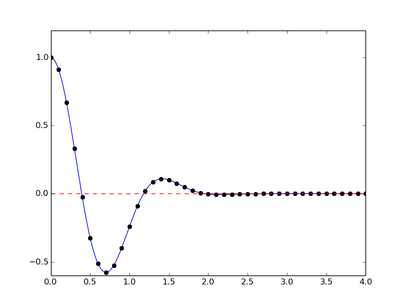
Running this program with some function, say \( f(x)=e^{-x^2}\cos(4x) \) (which has a solution at \( x = \frac{\pi}{8} \)), gives the root 0.392699, which has an error of \( 8.2\cdot 10^{-8} \). Increasing the number of points with a factor of ten gives a root with an error of \( 3.1\cdot 10^{-10} \).
After such a quick "flat" implementation of an algorithm, we should always try to offer the algorithm as a Matlab function, applicable to as wide a problem domain as possible. The function should take \( f \) and an associated interval \( [a,b] \) as input, as well as a number of points (\( n \)), and return a list of all the roots in \( [a,b] \). Here is our candidate for a good implementation of the brute force rooting finding algorithm:
function all_roots = brute_force_root_finder(f, a, b, n)
    x = linspace(a, b, n);
    y = f(x);
    roots = [];
    for i = 1:(n-1)
        if y(i)*y(i+1) < 0
            root = x(i) - (x(i+1) - x(i))/(y(i+1) - y(i))*y(i);
            roots = [roots; root];
        end
    end
    all_roots = roots;
end
This function is found in the file brute_force_root_finder.m.
This time we use another elegant technique to indicate if roots were found
or not: roots is empty (an array of length zero) if the root finding was unsuccessful,
otherwise it contains all the roots. Application of the function to
the previous example can be coded as
(demo_brute_force_root_finder.m):
function demo_brute_force_root_finder()
    roots = brute_force_root_finder(
        @(x) exp(-x.^2).*cos(4*x), 0, 4, 1001);
    if length(roots) > 0
        roots
    else
        fprintf('Could not find any roots');
    end
end
Brute force optimization
Numerical algorithm
We realize that \( x_i \) corresponds to a maximum point if \( y_{i-1} < y_i > y_{i+1} \). Similarly, \( x_i \) corresponds to a minimum if \( y_{i-1} > y_i < y_{i+1} \). We can do this test for all "inner" points \( i=1,\ldots,n-1 \) to find all local minima and maxima. In addition, we need to add an end point, \( i=0 \) or \( i=n \), if the corresponding \( y_i \) is a global maximum or minimum.
Implementation
The algorithm above can be translated to the following Matlab function (file brute_force_optimizer.m):
function [xy_minima, xy_maxima] = brute_force_optimizer(f, a, b, n)
    x = linspace(a, b, n);
    y = f(x);
    % Let maxima and minima hold the indices corresponding
    % to (local) maxima and minima points
    minima = [];
    maxima = [];
    for i = 2:(n-1)
        if y(i-1) < y(i) && y(i) > y(i+1)
            maxima = [maxima; i];
        end
        if y(i-1) > y(i) && y(i) < y(i+1)
            minima = [minima; i];
        end
    end

    % What about the end points?
    y_min_inner = y(minima(1));   % Initialize
    for i = 1:length(minima)
        if y(minima(i)) < y_min_inner
            y_min_inner = y(minima(i));
        end
    end
    y_max_inner = y(maxima(1));   % Initialize
    for i = 1:length(maxima)
        if y(maxima(i)) > y_max_inner
            y_max_inner = y(maxima(i));
        end
    end

    if y(1) > y_max_inner
        maxima = [maxima; 1];
    end
    if y(length(x)) > y_max_inner
       maxima = [maxima; length(x)];
    end
    if y(1) < y_min_inner
        minima = [minima; 1];
    end
    if y(length(x)) < y_min_inner
        minima = [minima; length(x)];
    end

    % Compose return values
    xy_minima = [];
    for i = 1:length(minima)
        xy_minima = [xy_minima; [x(minima(i)) y(minima(i))]];
    end
    xy_maxima = [];
    for i = 1:length(maxima)
        xy_maxima = [xy_maxima; [x(maxima(i)) y(maxima(i))]];
    end
end
An application to \( f(x)=e^{-x^2}\cos(4x) \) looks like
function demo_brute_force_optimizer
    [xy_minima, xy_maxima] = brute_force_optimizer(
        @(x) exp(-x.^2).*cos(4*x), 0, 4, 1001);
    xy_minima
    xy_maxima
end
Model problem for algebraic equations
We shall consider the very simple problem of finding the square root of 9, which is the positive solution of \( x^2=9 \). The nice feature of solving an equation whose solution is known beforehand is that we can easily investigate how the numerical method and the implementation perform in the search for the solution. The \( f(x) \) function corresponding to the equation \( x^2=9 \) is $$ f(x) = x^2 - 9\thinspace .$$ Our interval of interest for solutions will be \( [0,1000] \) (the upper limit here is chosen somewhat arbitrarily).
In the following, we will present several efficient and accurate methods for solving nonlinear algebraic equations, both single equation and systems of equations. The methods all have in common that they search for approximate solutions. The methods differ, however, in the way they perform the search for solutions. The idea for the search influences the efficiency of the search and the reliability of actually finding a solution. For example, Newton's method is very fast, but not reliable, while the bisection method is the slowest, but absolutely reliable. No method is best at all problems, so we need different methods for different problems.