Approximation of vectors

We shall start with introducing two fundamental methods for determining the coefficients \(c_i\) in (1.1) and illustrate the methods on approximation of vectors, because vectors in vector spaces give a more intuitive understanding than starting directly with approximation of functions in function spaces. The extension from vectors to functions will be trivial as soon as the fundamental ideas are understood.

The first method of approximation is called the least squares method and consists in finding \(c_i\) such that the difference \(u-f\), measured in some norm, is minimized. That is, we aim at finding the best approximation \(u\) to \(f\) (in some norm). The second method is not as intuitive: we find \(u\) such that the error \(u-f\) is orthogonal to the space where we seek \(u\). This is known as projection, or we may also call it a Galerkin method. When approximating vectors and functions, the two methods are equivalent, but this is no longer the case when applying the principles to differential equations.

Approximation of planar vectors

Suppose we have given a vector \(\boldsymbol{f} = (3,5)\) in the \(xy\) plane and that we want to approximate this vector by a vector aligned in the direction of the vector \((a,b)\). Figure Approximation of a two-dimensional vector by a one-dimensional vector depicts the situation.

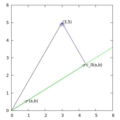
Approximation of a two-dimensional vector by a one-dimensional vector

We introduce the vector space \(V\) spanned by the vector \(\boldsymbol{\psi}_0=(a,b)\):

\[V = \mbox{span}\,\{ \boldsymbol{\psi}_0\}{\thinspace .}\]

We say that \(\boldsymbol{\psi}_0\) is a basis vector in the space \(V\). Our aim is to find the vector \(\boldsymbol{u} = c_0\boldsymbol{\psi}_0\in V\) which best approximates the given vector \(\boldsymbol{f} = (3,5)\). A reasonable criterion for a best approximation could be to minimize the length of the difference between the approximate \(\boldsymbol{u}\) and the given \(\boldsymbol{f}\). The difference, or error \(\boldsymbol{e} = \boldsymbol{f} -\boldsymbol{u}\), has its length given by the norm

\[||\boldsymbol{e}|| = (\boldsymbol{e},\boldsymbol{e})^{\frac{1}{2}},\]

where \((\boldsymbol{e},\boldsymbol{e})\) is the inner product of \(\boldsymbol{e}\) and itself. The inner product, also called scalar product or dot product, of two vectors \(\boldsymbol{u}=(u_0,u_1)\) and \(\boldsymbol{v} =(v_0,v_1)\) is defined as

\[(\boldsymbol{u}, \boldsymbol{v}) = u_0v_0 + u_1v_1{\thinspace .}\]

Remark 1. We should point out that we use the notation \((\cdot,\cdot)\) for two different things: \((a,b)\) for scalar quantities \(a\) and \(b\) means the vector starting in the origin and ending in the point \((a,b)\), while \((\boldsymbol{u},\boldsymbol{v})\) with vectors \(\boldsymbol{u}\) and \(\boldsymbol{v}\) means the inner product of these vectors. Since vectors are here written in boldface font there should be no confusion. We may add that the norm associated with this inner product is the usual Eucledian length of a vector.

Remark 2. It might be wise to refresh some basic linear algebra by consulting a textbook. Exercise 1: Linear algebra refresher I and Exercise 2: Linear algebra refresher II suggest specific tasks to regain familiarity with fundamental operations on inner product vector spaces.

The least squares method (1)

We now want to find \(c_0\) such that it minimizes \(||\boldsymbol{e}||\). The algebra is simplified if we minimize the square of the norm, \(||\boldsymbol{e}||^2 = (\boldsymbol{e}, \boldsymbol{e})\), instead of the norm itself. Define the function

\[E(c_0) = (\boldsymbol{e},\boldsymbol{e}) = (\boldsymbol{f} - c_0\boldsymbol{\psi}_0, \boldsymbol{f} - c_0\boldsymbol{\psi}_0) {\thinspace .}\]

We can rewrite the expressions of the right-hand side in a more convenient form for further work:

(1)\[ E(c_0) = (\boldsymbol{f},\boldsymbol{f}) - 2c_0(\boldsymbol{f},\boldsymbol{\psi}_0) + c_0^2(\boldsymbol{\psi}_0,\boldsymbol{\psi}_0){\thinspace .}\]

The rewrite results from using the following fundamental rules for inner product spaces:

(2)\[ (\alpha\boldsymbol{u},\boldsymbol{v})=\alpha(\boldsymbol{u},\boldsymbol{v}),\quad \alpha\in\mathbb{R},\]

(3)\[ (\boldsymbol{u} +\boldsymbol{v},\boldsymbol{w}) = (\boldsymbol{u},\boldsymbol{w}) + (\boldsymbol{v}, \boldsymbol{w}),\]

(4)\[ (\boldsymbol{u}, \boldsymbol{v}) = (\boldsymbol{v}, \boldsymbol{u}){\thinspace .}\]

Minimizing \(E(c_0)\) implies finding \(c_0\) such that

\[\frac{\partial E}{\partial c_0} = 0{\thinspace .}\]

Differentiating (1) with respect to \(c_0\) gives

(5)\[ \frac{\partial E}{\partial c_0} = -2(\boldsymbol{f},\boldsymbol{\psi}_0) + 2c_0 (\boldsymbol{\psi}_0,\boldsymbol{\psi}_0) {\thinspace .}\]

Setting the above expression equal to zero and solving for \(c_0\) gives

(6)\[ c_0 = \frac{(\boldsymbol{f},\boldsymbol{\psi}_0)}{(\boldsymbol{\psi}_0,\boldsymbol{\psi}_0)},\]

which in the present case with \(\boldsymbol{\psi}_0=(a,b)\) results in

\[c_0 = \frac{3a + 5b}{a^2 + b^2}{\thinspace .}\]

For later, it is worth mentioning that setting the key equation (5) to zero can be rewritten as

\[(\boldsymbol{f}-c0\boldsymbol{\psi}_0,\boldsymbol{\psi}_0) = 0,\]

or

(7)\[ (\boldsymbol{e}, \boldsymbol{\psi}_0) = 0 {\thinspace .}\]

The projection method

We shall now show that minimizing \(||\boldsymbol{e}||^2\) implies that \(\boldsymbol{e}\) is orthogonal to any vector \(\boldsymbol{v}\) in the space \(V\). This result is visually quite clear from Figure Approximation of a two-dimensional vector by a one-dimensional vector (think of other vectors along the line \((a,b)\): all of them will lead to a larger distance between the approximation and \(\boldsymbol{f}\)). To see this result mathematically, we express any \(\boldsymbol{v}\in V\) as \(\boldsymbol{v}=s\boldsymbol{\psi}_0\) for any scalar parameter \(s\), recall that two vectors are orthogonal when their inner product vanishes, and calculate the inner product

\[\begin{split}(\boldsymbol{e}, s\boldsymbol{\psi}_0) &= (\boldsymbol{f} - c_0\boldsymbol{\psi}_0, s\boldsymbol{\psi}_0)\\ &= (\boldsymbol{f},s\boldsymbol{\psi}_0) - (c_0\boldsymbol{\psi}_0, s\boldsymbol{\psi}_0)\\ &= s(\boldsymbol{f},\boldsymbol{\psi}_0) - sc_0(\boldsymbol{\psi}_0, \boldsymbol{\psi}_0)\\ &= s(\boldsymbol{f},\boldsymbol{\psi}_0) - s\frac{(\boldsymbol{f},\boldsymbol{\psi}_0)}{(\boldsymbol{\psi}_0,\boldsymbol{\psi}_0)}(\boldsymbol{\psi}_0,\boldsymbol{\psi}_0)\\ &= s\left( (\boldsymbol{f},\boldsymbol{\psi}_0) - (\boldsymbol{f},\boldsymbol{\psi}_0)\right)\\ &=0{\thinspace .}\end{split}\]

Therefore, instead of minimizing the square of the norm, we could demand that \(\boldsymbol{e}\) is orthogonal to any vector in \(V\). This method is known as projection, because it is the same as projecting the vector onto the subspace. (The approach can also be referred to as a Galerkin method as explained at the end of the section approximation!of general vectors.)

Mathematically the projection method is stated by the equation

(8)\[ (\boldsymbol{e}, \boldsymbol{v}) = 0,\quad\forall\boldsymbol{v}\in V{\thinspace .}\]

An arbitrary \(\boldsymbol{v}\in V\) can be expressed as \(s\boldsymbol{\psi}_0\), \(s\in\mathbb{R}\), and therefore (8) implies

\[(\boldsymbol{e},s\boldsymbol{\psi}_0) = s(\boldsymbol{e}, \boldsymbol{\psi}_0) = 0,\]

which means that the error must be orthogonal to the basis vector in the space \(V\):

\[(\boldsymbol{e}, \boldsymbol{\psi}_0)=0\quad\hbox{or}\quad (\boldsymbol{f} - c_0\boldsymbol{\psi}_0, \boldsymbol{\psi}_0)=0 {\thinspace .}\]

The latter equation gives (6) and it also arose from least squares computations in (7).

Approximation of general vectors

Let us generalize the vector approximation from the previous section to vectors in spaces with arbitrary dimension. Given some vector \(\boldsymbol{f}\), we want to find the best approximation to this vector in the space

\[V = \hbox{span}\,\{\boldsymbol{\psi}_0,\ldots,\boldsymbol{\psi}_N\} {\thinspace .}\]

We assume that the basis vectors \(\boldsymbol{\psi}_0,\ldots,\boldsymbol{\psi}_N\) are linearly independent so that none of them are redundant and the space has dimension \(N+1\). Any vector \(\boldsymbol{u}\in V\) can be written as a linear combination of the basis vectors,

\[\boldsymbol{u} = \sum_{j=0}^N c_j\boldsymbol{\psi}_j,\]

where \(c_j\in\mathbb{R}\) are scalar coefficients to be determined.

The least squares method (2)

Now we want to find \(c_0,\ldots,c_N\), such that \(\boldsymbol{u}\) is the best approximation to \(\boldsymbol{f}\) in the sense that the distance (error) \(\boldsymbol{e} = \boldsymbol{f} - \boldsymbol{u}\) is minimized. Again, we define the squared distance as a function of the free parameters \(c_0,\ldots,c_N\),

\[E(c_0,\ldots,c_N) = (\boldsymbol{e},\boldsymbol{e}) = (\boldsymbol{f} -\sum_jc_j\boldsymbol{\psi}_j,\boldsymbol{f} -\sum_jc_j\boldsymbol{\psi}_j) \nonumber\]

(9)\[ = (\boldsymbol{f},\boldsymbol{f}) - 2\sum_{j=0}^N c_j(\boldsymbol{f},\boldsymbol{\psi}_j) + \sum_{p=0}^N\sum_{q=0}^N c_pc_q(\boldsymbol{\psi}_p,\boldsymbol{\psi}_q){\thinspace .}\]

Minimizing this \(E\) with respect to the independent variables \(c_0,\ldots,c_N\) is obtained by requiring

\[\frac{\partial E}{\partial c_i} = 0,\quad i=0,\ldots,N {\thinspace .}\]

The second term in (9) is differentiated as follows:

\[\frac{\partial}{\partial c_i} \sum_{j=0}^N c_j(\boldsymbol{f},\boldsymbol{\psi}_j) = (\boldsymbol{f},\boldsymbol{\psi}_i),\]

since the expression to be differentiated is a sum and only one term, \(c_i(\boldsymbol{f},\boldsymbol{\psi}_i)\), contains \(c_i\) and this term is linear in \(c_i\). To understand this differentiation in detail, write out the sum specifically for, e.g, \(N=3\) and \(i=1\).

The last term in (9) is more tedious to differentiate. We start with

\[\frac{\partial}{\partial c_i} c_pc_q = \left\lbrace\begin{array}{ll} 0, \hbox{ if } p\neq i\hbox{ and } q\neq i,\]

\[c_q, \hbox{ if } p=i\hbox{ and } q\neq i,\]

\[c_p, \hbox{ if } p\neq i\hbox{ and } q=i,\]

\[2c_i, \hbox{ if } p=q= i,\]

\[\end{array}\right.\]

Then

\[\frac{\partial}{\partial c_i} \sum_{p=0}^N\sum_{q=0}^N c_pc_q(\boldsymbol{\psi}_p,\boldsymbol{\psi}_q) = \sum_{p=0, p\neq i}^N c_p(\boldsymbol{\psi}_p,\boldsymbol{\psi}_i) + \sum_{q=0, q\neq i}^N c_q(\boldsymbol{\psi}_q,\boldsymbol{\psi}_i) +2c_i(\boldsymbol{\psi}_i,\boldsymbol{\psi}_i){\thinspace .}\]

The last term can be included in the other two sums, resulting in

\[\frac{\partial}{\partial c_i} \sum_{p=0}^N\sum_{q=0}^N c_pc_q(\boldsymbol{\psi}_p,\boldsymbol{\psi}_q) = 2\sum_{j=0}^N c_i(\boldsymbol{\psi}_j,\boldsymbol{\psi}_i){\thinspace .}\]

It then follows that setting

\[\frac{\partial E}{\partial c_i} = 0,\quad i=0,\ldots,N,\]

leads to a linear system for \(c_0,\ldots,c_N\):

(10)\[ \sum_{j=0}^N A_{i,j} c_j = b_i, \quad i=0,\ldots,N,\]

where

\[A_{i,j} = (\boldsymbol{\psi}_i,\boldsymbol{\psi}_j),\]

\[b_i = (\boldsymbol{\psi}_i, \boldsymbol{f}){\thinspace .}\]

We have changed the order of the two vectors in the inner product according to (4):

\[A_{i,j} = (\boldsymbol{\psi}_j,\boldsymbol{\psi}_i) = (\boldsymbol{\psi}_i,\boldsymbol{\psi}_j),\]

simply because the sequence \(i\)-$j$ looks more aesthetic.

The Galerkin or projection method

In analogy with the “one-dimensional” example in the section Approximation of planar vectors, it holds also here in the general case that minimizing the distance (error) \(\boldsymbol{e}\) is equivalent to demanding that \(\boldsymbol{e}\) is orthogonal to all \(\boldsymbol{v}\in V\):

(11)\[ (\boldsymbol{e},\boldsymbol{v})=0,\quad \forall\boldsymbol{v}\in V{\thinspace .}\]

Since any \(\boldsymbol{v}\in V\) can be written as \(\boldsymbol{v} =\sum_{i=0}^N c_i\boldsymbol{\psi}_i\), the statement (11) is equivalent to saying that

\[(\boldsymbol{e}, \sum_{i=0}^N c_i\boldsymbol{\psi}_i) = 0,\]

for any choice of coefficients \(c_0,\ldots,c_N\). The latter equation can be rewritten as

\[\sum_{i=0}^N c_i (\boldsymbol{e},\boldsymbol{\psi}_i) =0{\thinspace .}\]

If this is to hold for arbitrary values of \(c_0,\ldots,c_N\) we must require that each term in the sum vanishes,

(12)\[ (\boldsymbol{e},\boldsymbol{\psi}_i)=0,\quad i=0,\ldots,N{\thinspace .}\]

These \(N+1\) equations result in the same linear system as (10):

\[(\boldsymbol{f} - \sum_{j=0}^N c_j\boldsymbol{\psi}_j, \boldsymbol{\psi}_i) = (\boldsymbol{f}, \boldsymbol{\psi}_i) - \sum_{j\in{\mathcal{I}_s}} (\boldsymbol{\psi}_i,\boldsymbol{\psi}_j)c_j = 0,\]

and hence

\[\sum_{j=0}^N (\boldsymbol{\psi}_i,\boldsymbol{\psi}_j)c_j = (\boldsymbol{f}, \boldsymbol{\psi}_i),\quad i=0,\ldots, N {\thinspace .}\]

So, instead of differentiating the \(E(c_0,\ldots,c_N)\) function, we could simply use (11) as the principle for determining \(c_0,\ldots,c_N\), resulting in the \(N+1\) equations (12).

The names least squares method or least squares approximation are natural since the calculations consists of minimizing \(||\boldsymbol{e}||^2\), and \(||\boldsymbol{e}||^2\) is a sum of squares of differences between the components in \(\boldsymbol{f}\) and \(\boldsymbol{u}\). We find \(\boldsymbol{u}\) such that this sum of squares is minimized.

The principle (11), or the equivalent form (12), is known as projection. Almost the same mathematical idea was used by the Russian mathematician Boris Galerkin to solve differential equations, resulting in what is widely known as Galerkin’s method.