Introduction to finite element methods
| Author: | Hans Petter Langtangen |
|---|---|
| Date: | Dec 16, 2013 |
PRELIMINARY VERSION
The finite element method is a powerful tool for solving differential equations. The method can easily deal with complex geometries and higher-order approximations of the solution. Figure Domain for flow around a dolphin shows a two-dimensional domain with a non-trivial geometry. The idea is to divide the domain into triangles (elements) and seek a polynomial approximations to the unknown functions on each triangle. The method glues these piecewise approximations together to find a global solution. Linear and quadratic polynomials over the triangles are particularly popular.
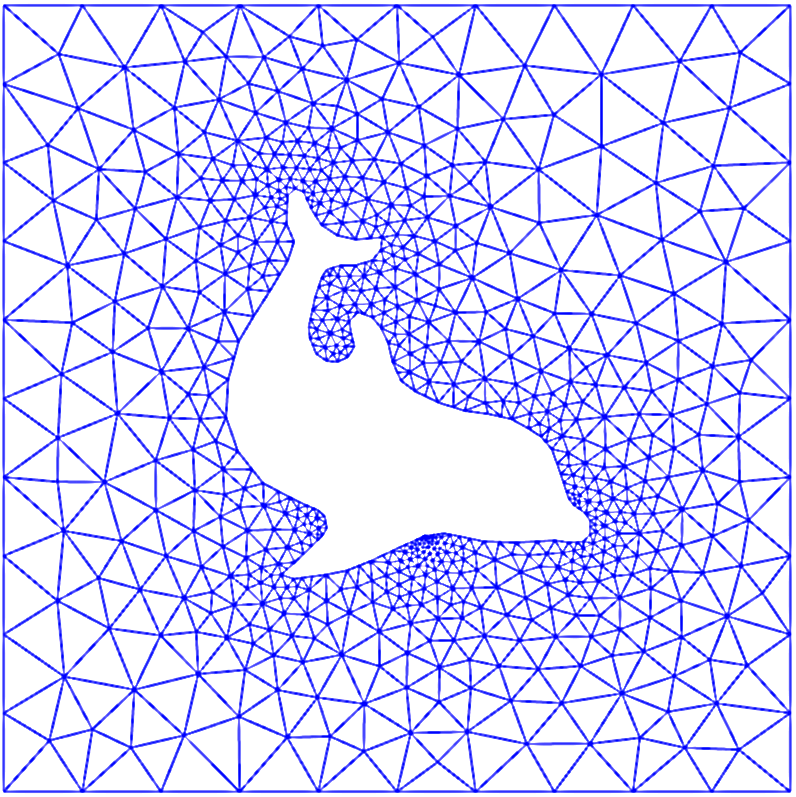
Domain for flow around a dolphin
Many successful numerical methods for differential equations, including the finite element method, aim at approximating the unknown function by a sum
where \({\psi}_i(x)\) are prescribed functions and \(c_0,\ldots,c_N\) are unknown coefficients to be determined. Solution methods for differential equations utilizing (1) must have a principle for constructing \(N+1\) equations to determine \(c_0,\ldots,c_N\). Then there is a machinery regarding the actual constructions of the equations for \(c_0,\ldots,c_N\), in a particular problem. Finally, there is a solve phase for computing the solution \(c_0,\ldots,c_N\) of the \(N+1\) equations.
Especially in the finite element method, the machinery for constructing the discrete equations to be implemented on a computer is quite comprehensive, with many mathematical and implementational details entering the scene at the same time. From an ease-of-learning perspective it can therefore be wise to introduce the computational machinery for a trivial equation: \(u=f\). Solving this equation with \(f\) given and \(u\) on the form (1) means that we seek an approximation \(u\) to \(f\). This approximation problem has the advantage of introducing most of the finite element toolbox, but with postponing demanding topics related to differential equations (e.g., integration by parts, boundary conditions, and coordinate mappings). This is the reason why we shall first become familiar with finite element approximation before addressing finite element methods for differential equations.
First, we refresh some linear algebra concepts about approximating vectors in vector spaces. Second, we extend these concepts to approximating functions in function spaces, using the same principles and the same notation. We present examples on approximating functions by global basis functions with support throughout the entire domain. Third, we introduce the finite element type of local basis functions and explain the computational algorithms for working with such functions. Three types of approximation principles are covered: 1) the least squares method, 2) the \(L_2\) projection or Galerkin method, and 3) interpolation or collocation.
