Implementation (1)
Goal
We want make a computer program for solving
by finite difference methods. The program should also display the numerical solution as a curve on the screen, preferably together with the exact solution. We shall also be concerned with program testing, user interfaces, and computing convergence rates.
All programs referred to in this section are found in the src/decay directory (we use the classical Unix term directory for what many others nowadays call folder).
Mathematical problem. We want to explore the Forward Euler scheme, the Backward Euler, and the Crank-Nicolson schemes applied to our model problem. From an implementational point of view, it is advantageous to implement the \(\theta\)-rule
since it can generate the three other schemes by various of choices of \(\theta\): \(\theta=0\) for Forward Euler, \(\theta =1\) for Backward Euler, and \(\theta =1/2\) for Crank-Nicolson. Given \(a\), \(u^0=I\), \(T\), and \(\Delta t\), our task is to use the \(\theta\)-rule to compute \(u^1, u^2,\ldots,u^{N_t}\), where \(t_{N_t}=N_t\Delta t\), and \(N_t\) the closest integer to \(T/\Delta t\).
Computer Language: Python. Any programming language can be used to generate the \(u^{n+1}\) values from the formula above. However, in this document we shall mainly make use of Python of several reasons:
- Python has a very clean, readable syntax (often known as “executable pseudo-code”).
- Python code is very similar to MATLAB code (and MATLAB has a particularly widespread use for scientific computing).
- Python is a full-fledged, very powerful programming language.
- Python is similar to, but much simpler to work with and results in more reliable code than C++.
- Python has a rich set of modules for scientific computing, and its popularity in scientific computing is rapidly growing.
- Python was made for being combined with compiled languages (C, C++, Fortran) to reuse existing numerical software and to reach high computational performance of new implementations.
- Python has extensive support for administrative task needed when doing large-scale computational investigations.
- Python has extensive support for graphics (visualization, user interfaces, web applications).
- FEniCS, a very powerful tool for solving PDEs by the finite element method, is most human-efficient to operate from Python.
Learning Python is easy. Many newcomers to the language will probably learn enough from the forthcoming examples to perform their own computer experiments. The examples start with simple Python code and gradually make use of more powerful constructs as we proceed. As long as it is not inconvenient for the problem at hand, our Python code is made as close as possible to MATLAB code for easy transition between the two languages.
Readers who feel the Python examples are too hard to follow will probably benefit from read a tutorial, e.g.,
The author also has a book [Ref1] that introduces scientific programming with Python.
Making a solver function
We choose to have an array u for storing the \(u^n\) values, \(n=0,1,\ldots,N_t\). The algorithmic steps are
- initialize \(u^0\)
- for \(t=t_n\), \(n=1,2,\ldots,N_t\): compute \(u_n\) using the \(\theta\)-rule formula
Function for computing the numerical solution
The following Python function takes the input data of the problem (\(I\), \(a\), \(T\), \(\Delta t\), \(\theta\)) as arguments and returns two arrays with the solution \(u^0,\ldots,u^{N_t}\) and the mesh points \(t_0,\ldots,t_{N_t}\), respectively:
from numpy import *

def solver(I, a, T, dt, theta):
    """Solve u'=-a*u, u(0)=I, for t in (0,T] with steps of dt."""
    Nt = int(T/dt)            # no of time intervals
    T = Nt*dt                 # adjust T to fit time step dt
    u = zeros(Nt+1)           # array of u[n] values
    t = linspace(0, T, Nt+1)  # time mesh

    u[0] = I                  # assign initial condition
    for n in range(0, Nt):    # n=0,1,...,Nt-1
        u[n+1] = (1 - (1-theta)*a*dt)/(1 + theta*dt*a)*u[n]
    return u, t
The numpy library contains a lot of functions for array computing. Most of the function names are similar to what is found in the alternative scientific computing language MATLAB. Here we make use of
- zeros(Nt+1) for creating an array of a size Nt+1 and initializing the elements to zero
- linspace(0, T, Nt+1) for creating an array with Nt+1 coordinates uniformly distributed between 0 and T
The for loop deserves a comment, especially for newcomers to Python. The construction range(0, Nt, s) generates all integers from 0 to Nt in steps of s, but not including Nt. Omitting s means s=1. For example, range(0, 6, 3) gives 0 and 3, while range(0, Nt) generates 0, 1, ..., Nt-1. Our loop implies the following assignments to u[n+1]: u[1], u[2], ..., u[Nt], which is what we want since u has length Nt+1. The first index in Python arrays or lists is always 0 and the last is then len(u)-1. The length of an array u is obtained by len(u) or u.size.
To compute with the solver function, we need to call it. Here is a sample call:
u, t = solver(I=1, a=2, T=8, dt=0.8, theta=1)
Integer division
The shown implementation of the solver may face problems and wrong results if T, a, dt, and theta are given as integers, see Exercise 4: Experiment with integer division and Exercise 5: Experiment with wrong computations. The problem is related to integer division in Python (as well as in Fortran, C, C++, and many other computer languages): 1/2 becomes 0, while 1.0/2, 1/2.0, or 1.0/2.0 all become 0.5. It is enough that at least the nominator or the denominator is a real number (i.e., a float object) to ensure correct mathematical division. Inserting a conversion dt = float(dt) guarantees that dt is float and avoids problems in Exercise 5: Experiment with wrong computations.
Another problem with computing \(N_t=T/\Delta t\) is that we should round \(N_t\) to the nearest integer. With Nt = int(T/dt) the int operation picks the largest integer smaller than T/dt. Correct mathematical rounding as known from school is obtained by
Nt = int(round(T/dt))
The complete version of our improved, safer solver function then becomes
from numpy import *

def solver(I, a, T, dt, theta):
    """Solve u'=-a*u, u(0)=I, for t in (0,T] with steps of dt."""
    dt = float(dt)            # avoid integer division
    Nt = int(round(T/dt))     # no of time intervals
    T = Nt*dt                 # adjust T to fit time step dt
    u = zeros(Nt+1)           # array of u[n] values
    t = linspace(0, T, Nt+1)  # time mesh

    u[0] = I                  # assign initial condition
    for n in range(0, Nt):    # n=0,1,...,Nt-1
        u[n+1] = (1 - (1-theta)*a*dt)/(1 + theta*dt*a)*u[n]
    return u, t
Doc strings
Right below the header line in the solver function there is a Python string enclosed in triple double quotes """. The purpose of this string object is to document what the function does and what the arguments are. In this case the necessary documentation do not span more than one line, but with triple double quoted strings the text may span several lines:
def solver(I, a, T, dt, theta):
    """
    Solve

        u'(t) = -a*u(t),

    with initial condition u(0)=I, for t in the time interval
    (0,T]. The time interval is divided into time steps of
    length dt.

    theta=1 corresponds to the Backward Euler scheme, theta=0
    to the Forward Euler scheme, and theta=0.5 to the Crank-
    Nicolson method.
    """
    ...
Such documentation strings appearing right after the header of a function are called doc strings. There are tools that can automatically produce nicely formatted documentation by extracting the definition of functions and the contents of doc strings.
It is strongly recommended to equip any function whose purpose is not obvious with a doc string. Nevertheless, the forthcoming text deviates from this rule if the function is explained in the text.
Formatting of numbers
Having computed the discrete solution u, it is natural to look at the numbers:
# Write out a table of t and u values:
for i in range(len(t)):
    print t[i], u[i]
This compact print statement gives unfortunately quite ugly output because the t and u values are not aligned in nicely formatted columns. To fix this problem, we recommend to use the printf format, supported most programming languages inherited from C. Another choice is Python’s recent format string syntax.
Writing t[i] and u[i] in two nicely formatted columns is done like this with the printf format:
print 't=%6.3f u=%g' % (t[i], u[i])
The percentage signs signify “slots” in the text where the variables listed at the end of the statement are inserted. For each “slot” one must specify a format for how the variable is going to appear in the string: s for pure text, d for an integer, g for a real number written as compactly as possible, 9.3E for scientific notation with three decimals in a field of width 9 characters (e.g., -1.351E-2), or .2f for standard decimal notation with two decimals formatted with minimum width. The printf syntax provides a quick way of formatting tabular output of numbers with full control of the layout.
The alternative format string syntax looks like
print 't={t:6.3f} u={u:g}'.format(t=t[i], u=u[i])
As seen, this format allows logical names in the “slots” where t[i] and u[i] are to be inserted. The “slots” are surrounded by curly braces, and the logical name is followed by a colon and then the printf-like specification of how to format real numbers, integers, or strings.
Running the program
The function and main program shown above must be placed in a file, say with name decay_v1.py (v1 stands for “version 1” - we shall make numerous different versions of this program). Make sure you write the code with a suitable text editor (Gedit, Emacs, Vim, Notepad++, or similar). The program is run by executing the file this way:
Terminal> python decay_v1.py
The text Terminal> just indicates a prompt in a Unix/Linux or DOS terminal window. After this prompt, which will look different in your terminal window, depending on the terminal application and how it is set up, commands like python decay_v1.py can be issued. These commands are interpreted by the operating system.
We strongly recommend to run Python programs within the IPython shell. First start IPython by typing ipython in the terminal window. Inside the IPython shell, our program decay_v1.py is run by the command run decay_v1.py:
Terminal> ipython

In [1]: run decay_v1.py
t= 0.000 u=1
t= 0.800 u=0.384615
t= 1.600 u=0.147929
t= 2.400 u=0.0568958
t= 3.200 u=0.021883
t= 4.000 u=0.00841653
t= 4.800 u=0.00323713
t= 5.600 u=0.00124505
t= 6.400 u=0.000478865
t= 7.200 u=0.000184179
t= 8.000 u=7.0838e-05

In [2]:
The advantage of running programs in IPython are many: previous commands are easily recalled with the up arrow, %pdb turns on debugging so that variables can be examined if the program aborts due to an exception, output of commands are stored in variables, programs and statements can be profiled, any operating system command can be executed, modules can be loaded automatically and other customizations can be performed when starting IPython – to mention a few of the most useful features.
Although running programs in IPython is strongly recommended, most execution examples in the forthcoming text use the standard Python shell with prompt >>> and run programs through a typesetting like
Terminal> python programname
The reason is that such typesetting makes the text more compact in the vertical direction than showing sessions with IPython syntax.
Verifying the implementation
It is easy to make mistakes while deriving and implementing numerical algorithms, so we should never believe in the printed \(u\) values before they have been thoroughly verified. The most obvious idea is to compare the computed solution with the exact solution, when that exists, but there will always be a discrepancy between these two solutions because of the numerical approximations. The challenging question is whether we have the mathematically correct discrepancy or if we have another, maybe small, discrepancy due to both an approximation error and an error in the implementation.
The purpose of verifying a program is to bring evidence for the property that there are no errors in the implementation. To avoid mixing unavoidable approximation errors and undesired implementation errors, we should try to make tests where we have some exact computation of the discrete solution or at least parts of it. Examples will show how this can be done.
Running a few algorithmic steps by hand
The simplest approach to produce a correct reference for the discrete solution \(u\) of finite difference equations is to compute a few steps of the algorithm by hand. Then we can compare the hand calculations with numbers produced by the program.
A straightforward approach is to use a calculator and compute \(u^1\), \(u^2\), and \(u^3\). With \(I=0.1\), \(\theta=0.8\), and \(\Delta t =0.8\) we get
Comparison of these manual calculations with the result of the solver function is carried out in the function
def verify_three_steps():
    """Compare three steps with known manual computations."""
    theta = 0.8; a = 2; I = 0.1; dt = 0.8
    u_by_hand = array([I,
                       0.0298245614035,
                       0.00889504462912,
                       0.00265290804728])

    Nt = 3  # number of time steps
    u, t = solver(I=I, a=a, T=Nt*dt, dt=dt, theta=theta)

    tol = 1E-15  # tolerance for comparing floats
    difference = abs(u - u_by_hand).max()
    success = difference <= tol
    return success
The main program, where we call the solver function and print u, is now put in a separate function main:
def main():
    u, t = solver(I=1, a=2, T=8, dt=0.8, theta=1)
    # Write out a table of t and u values:
    for i in range(len(t)):
        print 't=%6.3f u=%g' % (t[i], u[i])
        # or print 't={t:6.3f} u={u:g}'.format(t=t[i], u=u[i])
The main program in the file may now first run the verification test and then go on with the real simulation (main()) only if the test is passed:
if verify_three_steps():
    main()
else:
    print 'Bug in the implementation!'
Since the verification test is always done, future errors introduced accidentally in the program have a good chance of being detected.
Caution: choice of parameter values
For the choice of values of parameters in verification tests one should stay away from integers, especially 0 and 1, as these can simplify formulas too much for test purposes. For example, with \(\theta =1\) the nominator in the formula for \(u^n\) will be the same for all \(a\) and \(\Delta t\) values. One should therefore choose more “arbitrary” values, say \(\theta =0.8\) and \(I=0.1\).
It is essential that verification tests can be automatically run at any time. For this purpose, there are test frameworks and corresponding programming rules that allow us to request running through a suite of test cases (see the section Unit testing with nose), but in this very early stage of program development we just implement and run the verification in our own code so that every detail is visible and understood.
The complete program including the verify_three_steps* functions is found in the file decay_verf1.py (verf1 is a short name for “verification, version 1”).
Comparison with an exact discrete solution
Sometimes it is possible to find a closed-form exact discrete solution that fulfills the discrete finite difference equations. The implementation can then be verified against the exact discrete solution. This is usually the best technique for verification.
Define
Manual computations with the \(\theta\)-rule results in
We have then established the exact discrete solution as
Caution
One should be conscious about the different meanings of the notation on the left- and right-hand side of (1): on the left, \(n\) in \(u^n\) is a superscript reflecting a counter of mesh points (\(t_n\)), while on the right, \(n\) is the power in the exponentiation \(A^n\).
Comparison of the exact discrete solution and the computed solution is done in the following function:
def verify_exact_discrete_solution():

    def exact_discrete_solution(n, I, a, theta, dt):
        A = (1 - (1-theta)*a*dt)/(1 + theta*dt*a)
        return I*A**n

    theta = 0.8; a = 2; I = 0.1; dt = 0.8
    Nt = int(8/dt)  # no of steps
    u, t = solver(I=I, a=a, T=Nt*dt, dt=dt, theta=theta)
    u_de = array([exact_discrete_solution(n, I, a, theta, dt)
                  for n in range(Nt+1)])
    difference = abs(u_de - u).max()  # max deviation
    tol = 1E-15  # tolerance for comparing floats
    success = difference <= tol
    return success
The complete program is found in the file decay_verf2.py (verf2 is a short name for “verification, version 2”).
Local functions
One can define a function inside another function, here called a local function (also known as closure) inside a parent function. A local function is invisible outside the parent function. A convenient property is that any local function has access to all variables defined in the parent function, also if we send the local function to some other function as argument (!). In the present example, it means that the local function exact_discrete_solution does not need its five arguments as the values can alternatively be accessed through the local variables defined in the parent function verify_exact_discrete_solution. We can send such an exact_discrete_solution without arguments to any other function and exact_discrete_solution will still have access to n, I, a, and so forth defined in its parent function.
Computing the numerical error as a mesh function
Now that we have evidence for a correct implementation, we are in a position to compare the computed \(u^n\) values in the u array with the exact \(u\) values at the mesh points, in order to study the error in the numerical solution.
Let us first make a function for the analytical solution \({u_{\small\mbox{e}}}(t)=Ie^{-at}\) of the model problem:
def exact_solution(t, I, a):
    return I*exp(-a*t)
A natural way to compare the exact and discrete solutions is to calculate their difference as a mesh function:
We may view \({u_{\small\mbox{e}}}^n = {u_{\small\mbox{e}}}(t_n)\) as the representation of \({u_{\small\mbox{e}}}(t)\) as a mesh function rather than a continuous function defined for all \(t\in [0,T]\) (\({u_{\small\mbox{e}}}^n\) is often called the representative of \({u_{\small\mbox{e}}}\) on the mesh). Then, \(e^n = {u_{\small\mbox{e}}}^n - u^n\) is clearly the difference of two mesh functions. This interpretation of \(e^n\) is natural when programming.
The error mesh function \(e^n\) can be computed by
u, t = solver(I, a, T, dt, theta)  # Numerical sol.
u_e = exact_solution(t, I, a)      # Representative of exact sol.
e = u_e - u
Note that the mesh functions u and u_e are represented by arrays and associated with the points in the array t.
Array arithmetics
The last statements
u_e = exact_solution(t, I, a)
e = u_e - u
are primary examples of array arithmetics: t is an array of mesh points that we pass to exact_solution. This function evaluates -a*t, which is a scalar times an array, meaning that the scalar is multiplied with each array element. The result is an array, let us call it tmp1. Then exp(tmp1) means applying the exponential function to each element in tmp, resulting an array, say tmp2. Finally, I*tmp2 is computed (scalar times array) and u_e refers to this array returned from exact_solution. The expression u_e - u is the difference between two arrays, resulting in a new array referred to by e.
Computing the norm of the numerical error
Instead of working with the error \(e^n\) on the entire mesh, we often want one number expressing the size of the error. This is obtained by taking the norm of the error function.
Let us first define norms of a function \(f(t)\) defined for all \(t\in [0,T]\). Three common norms are
The \(L^2\) norm (2) (“L-two norm”) has nice mathematical properties and is the most popular norm. It is a generalization of the well-known Eucledian norm of vectors to functions. The \(L^\infty\) is also called the max norm or the supremum norm. In fact, there is a whole family of norms,
with \(p\) real. In particular, \(p=1\) corresponds to the \(L^1\) norm above while \(p=\infty\) is the \(L^\infty\) norm.
Numerical computations involving mesh functions need corresponding norms. Given a set of function values, \(f^n\), and some associated mesh points, \(t_n\), a numerical integration rule can be used to calculate the \(L^2\) and \(L^1\) norms defined above. Imagining that the mesh function is extended to vary linearly between the mesh points, the Trapezoidal rule is in fact an exact integration rule. A possible modification of the \(L^2\) norm for a mesh function \(f^n\) on a uniform mesh with spacing \(\Delta t\) is therefore the well-known Trapezoidal integration formula
A common approximation of this expression, motivated by the convenience of having a simpler formula, is
This is called the discrete \(L^2\) norm and denoted by \(\ell^2\). The error in \(||f||_{\ell^2}^2\) compared with the Trapezoidal integration formula is \(\Delta t((f^0)^2 + (f^{N_t})^2)/2\), which means perturbed weights at the end points of the mesh function, and the error goes to zero as \(\Delta t\rightarrow 0\). As long as we are consistent and stick to one kind of integration rule for the norm of a mesh function, the details and accuracy of this rule is not of concern.
The three discrete norms for a mesh function \(f^n\), corresponding to the \(L^2\), \(L^1\), and \(L^\infty\) norms of \(f(t)\) defined above, are defined by
Note that the \(L^2\), \(L^1\), \(\ell^2\), and \(\ell^1\) norms depend on the length of the interval of interest (think of \(f=1\), then the norms are proportional to \(\sqrt{T}\) or \(T\)). In some applications it is convenient to think of a mesh function as just a vector of function values and neglect the information of the mesh points. Then we can replace \(\Delta t\) by \(T/N_t\) and drop \(T\). Moreover, it is convenient to divide by the total length of the vector, \(N_t+1\), instead of \(N_t\). This reasoning gives rise to the vector norms for a vector \(f=(f_0,\ldots,f_{N})\):
Here we have used the common vector component notation with subscripts (\(f_n\)) and \(N\) as length. We will mostly work with mesh functions and use the discrete \(\ell^2\) norm (5) or the max norm \(\ell^\infty\) (7), but the corresponding vector norms (8)-(10) are also much used in numerical computations, so it is important to know the different norms and the relations between them.
A single number that expresses the size of the numerical error will be taken as \(||e^n||_{\ell^2}\) and called \(E\):
The corresponding Python code, using array arithmetics, reads
E = sqrt(dt*sum(e**2))
The sum function comes from numpy and computes the sum of the elements of an array. Also the sqrt function is from numpy and computes the square root of each element in the array argument.
Scalar computing
Instead of doing array computing sqrt(dt*sum(e**2)) we can compute with one element at a time:
m = len(u)     # length of u array (alt: u.size)
u_e = zeros(m)
t = 0
for i in range(m):
    u_e[i] = exact_solution(t, a, I)
    t = t + dt
e = zeros(m)
for i in range(m):
    e[i] = u_e[i] - u[i]
s = 0  # summation variable
for i in range(m):
    s = s + e[i]**2
error = sqrt(dt*s)
Such element-wise computing, often called scalar computing, takes more code, is less readable, and runs much slower than what we can achieve with array computing.
Plotting solutions
Having the t and u arrays, the approximate solution u is visualized by the intuitive command plot(t, u):
from matplotlib.pyplot import *
plot(t, u)
show()
Plotting multiple curves
It will be illustrative to also plot \({u_{\small\mbox{e}}}(t)\) for comparison. Doing a plot(t, u_e) is not exactly what we want: the plot function draws straight lines between the discrete points (t[n], u_e[n]) while \({u_{\small\mbox{e}}}(t)\) varies as an exponential function between the mesh points. The technique for showing the “exact” variation of \({u_{\small\mbox{e}}}(t)\) between the mesh points is to introduce a very fine mesh for \({u_{\small\mbox{e}}}(t)\):
t_e = linspace(0, T, 1001)      # fine mesh
u_e = exact_solution(t_e, I, a)
plot(t_e, u_e, 'b-')            # blue line for u_e
plot(t,   u,   'r--o')          # red dashes w/circles
With more than one curve in the plot we need to associate each curve with a legend. We also want appropriate names on the axis, a title, and a file containing the plot as an image for inclusion in reports. The Matplotlib package (matplotlib.pyplot) contains functions for this purpose. The names of the functions are similar to the plotting functions known from MATLAB. A complete plot session then becomes
from matplotlib.pyplot import *

figure()                          # create new plot
t_e = linspace(0, T, 1001)        # fine mesh for u_e
u_e = exact_solution(t_e, I, a)
plot(t,   u,   'r--o')            # red dashes w/circles
plot(t_e, u_e, 'b-')              # blue line for exact sol.
legend(['numerical', 'exact'])
xlabel('t')
ylabel('u')
title('theta=%g, dt=%g' % (theta, dt))
savefig('%s_%g.png' % (theta, dt))
show()
Note that savefig here creates a PNG file whose name reflects the values of \(\theta\) and \(\Delta t\) so that we can easily distinguish files from different runs with \(\theta\) and \(\Delta t\).
A bit more sophisticated and easy-to-read filename can be generated by mapping the \(\theta\) value to acronyms for the three common schemes: FE (Forward Euler, \(\theta=0\)), BE (Backward Euler, \(\theta=1\)), CN (Crank-Nicolson, \(\theta=0.5\)). A Python dictionary is ideal for such a mapping from numbers to strings:
theta2name = {0: 'FE', 1: 'BE', 0.5: 'CN'}
savefig('%s_%g.png' % (theta2name[theta], dt))
Experiments with computing and plotting
Let us wrap up the computation of the error measure and all the plotting statements in a function explore. This function can be called for various \(\theta\) and \(\Delta t\) values to see how the error varies with the method and the mesh resolution:
def explore(I, a, T, dt, theta=0.5, makeplot=True):
    """
    Run a case with the solver, compute error measure,
    and plot the numerical and exact solutions (if makeplot=True).
    """
    u, t = solver(I, a, T, dt, theta)    # Numerical solution
    u_e = exact_solution(t, I, a)
    e = u_e - u
    E = sqrt(dt*sum(e**2))
    if makeplot:
        figure()                         # create new plot
        t_e = linspace(0, T, 1001)       # fine mesh for u_e
        u_e = exact_solution(t_e, I, a)
        plot(t,   u,   'r--o')           # red dashes w/circles
        plot(t_e, u_e, 'b-')             # blue line for exact sol.
        legend(['numerical', 'exact'])
        xlabel('t')
        ylabel('u')
        title('theta=%g, dt=%g' % (theta, dt))
        theta2name = {0: 'FE', 1: 'BE', 0.5: 'CN'}
        savefig('%s_%g.png' % (theta2name[theta], dt))
        savefig('%s_%g.pdf' % (theta2name[theta], dt))
        savefig('%s_%g.eps' % (theta2name[theta], dt))
        show()
    return E
The figure() call is key here: without it, a new plot command will draw the new pair of curves in the same plot window, while we want the different pairs to appear in separate windows and files. Calling figure() ensures this.
The explore function stores the plot in three different image file formats: PNG, PDF, and EPS (Encapsulated PostScript). The PNG format is aimed at being included in HTML files, the PDF format in pdfLaTeX documents, and the EPS format in LaTeX documents. Frequently used viewers for these image files on Unix systems are gv (comes with Ghostscript) for the PDF and EPS formats and display (from the ImageMagick) suite for PNG files:
Terminal> gv BE_0.5.pdf
Terminal> gv BE_0.5.eps
Terminal> display BE_0.5.png
The complete code containing the functions above resides in the file decay_plot_mpl.py. Running this program results in
Terminal> python decay_plot_mpl.py
0.0   0.40:    2.105E-01
0.0   0.04:    1.449E-02
0.5   0.40:    3.362E-02
0.5   0.04:    1.887E-04
1.0   0.40:    1.030E-01
1.0   0.04:    1.382E-02
We observe that reducing \(\Delta t\) by a factor of 10 increases the accuracy for all three methods (\(\theta\) values). We also see that the combination of \(\theta=0.5\) and a small time step \(\Delta t =0.04\) gives a much more accurate solution, and that \(\theta=0\) and \(\theta=1\) with \(\Delta t = 0.4\) result in the least accurate solutions.
Figure The Forward Euler scheme for two values of the time step demonstrates that the numerical solution for \(\Delta t=0.4\) clearly lies below the exact curve, but that the accuracy improves considerably by reducing the time step by a factor of 10.
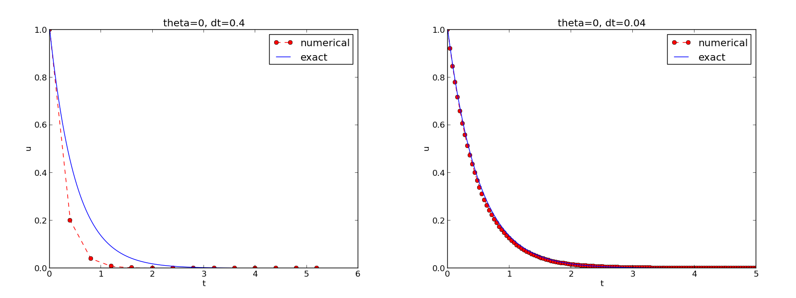
The Forward Euler scheme for two values of the time step
Combining plot files (1)
Mounting two PNG files, as done in the figure, is easily done by the montage program from the ImageMagick suite:
Terminal> montage -background white -geometry 100% -tile 2x1 \
          FE_0.4.png FE_0.04.png FE1.png
Terminal> convert -trim FE1.png FE1.png
The -geometry argument is used to specify the size of the image, and here we preserve the individual sizes of the images. The -tile HxV option specifies H images in the horizontal direction and V images in the vertical direction. A series of image files to be combined are then listed, with the name of the resulting combined image, here FE1.png at the end. The convert -trim command removes surrounding white areas in the figure (an operation usually known as cropping in image manipulation programs).
For LaTeX{} reports it is not recommended to use montage and PNG files as the result has too low resolution. Instead, plots should be made in the PDF format and combined using the pdftk, pdfnup, and pdfcrop tools (on Linux/Unix):
Terminal> pdftk FE_0.4.png FE_0.04.png output tmp.pdf
Terminal> pdfnup --nup 2x1 tmp.pdf     # output in tmp-nup.pdf
Terminal> pdfcrop tmp-nup.pdf FE1.png  # output in FE1.png
Here, pdftk combines images into a multi-page PDF file, pdfnup combines the images in individual pages to a table of images (pages), and pdfcrop removes white margins in the resulting combined image file.
The behavior of the two other schemes is shown in Figures The Backward Euler scheme for two values of the time step and The Crank-Nicolson scheme for two values of the time step. Crank-Nicolson is obviously the most accurate scheme from this visual point of view.
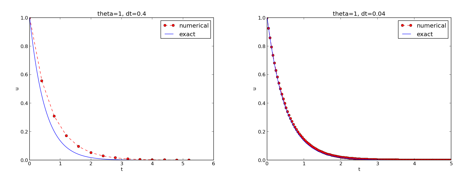
The Backward Euler scheme for two values of the time step

The Crank-Nicolson scheme for two values of the time step
Plotting with SciTools
The SciTools package provides a unified plotting interface, called Easyviz, to many different plotting packages, including Matplotlib, Gnuplot, Grace, MATLAB, VTK, OpenDX, and VisIt. The syntax is very similar to that of Matplotlib and MATLAB. In fact, the plotting commands shown above look the same in SciTool’s Easyviz interface, apart from the import statement, which reads
from scitools.std import *
This statement performs a from numpy import * as well as an import of the most common pieces of the Easyviz (scitools.easyviz) package, along with some additional numerical functionality.
With Easyviz one can merge several plotting commands into a single one using keyword arguments:
plot(t,   u,   'r--o',           # red dashes w/circles
     t_e, u_e, 'b-',             # blue line for exact sol.
     legend=['numerical', 'exact'],
     xlabel='t',
     ylabel='u',
     title='theta=%g, dt=%g' % (theta, dt),
     savefig='%s_%g.png' % (theta2name[theta], dt),
     show=True)
The decay_plot_st.py file contains such a demo.
By default, Easyviz employs Matplotlib for plotting, but Gnuplot and Grace are viable alternatives:
Terminal> python decay_plot_st.py --SCITOOLS_easyviz_backend gnuplot
Terminal> python decay_plot_st.py --SCITOOLS_easyviz_backend grace
The backend used for creating plots (and numerous other options) can be permanently set in SciTool’s configuration file.
All the Gnuplot windows are launched without any need to kill one before the next one pops up (as is the case with Matplotlib) and one can press the key ‘q’ anywhere in a plot window to kill it. Another advantage of Gnuplot is the automatic choice of sensible and distinguishable line types in black-and-white PDF and PostScript files.
Regarding functionality for annotating plots with title, labels on the axis, legends, etc., we refer to the documentation of Matplotlib and SciTools for more detailed information on the syntax. The hope is that the programming syntax explained so far suffices for understanding the code and learning more from a combination of the forthcoming examples and other resources such as books and web pages.
Test the understanding
Exercise 2: Implement schemes for Newton’s law of cooling asks you to implement a solver for a problem that is slightly different from the one above. You may use the solver and explore functions explained above as a starting point. Apply the new solver to Exercise 3: Find time of murder from body temperature.
Creating command-line interfaces
It is good programming practice to let programs read input from the user rather than require the user to edit the source code when trying out new values of input parameters. Reading input from the command line is a simple and flexible way of interacting with the user. Python stores all the command-line arguments in the list sys.argv, and there are, in principle, two ways of programming with command-line arguments in Python:
- Decide upon a sequence of parameters on the command line and read their values directly from the sys.argv[1:] list (sys.argv[0] is the just program name).
- Use option-value pairs (--option value) on the command line to override default values of input parameters, and utilize the argparse.ArgumentParser tool to interact with the command line.
Both strategies will be illustrated next.
Reading a sequence of command-line arguments
The decay_plot_mpl.py program needs the following input data: \(I\), \(a\), \(T\), an option to turn the plot on or off (makeplot), and a list of \(\Delta t\) values.
The simplest way of reading this input from the command line is to say that the first four command-line arguments correspond to the first four points in the list above, in that order, and that the rest of the command-line arguments are the \(\Delta t\) values. The input given for makeplot can be a string among 'on', 'off', 'True', and 'False'. The code for reading this input is most conveniently put in a function:
import sys

def read_command_line():
    if len(sys.argv) < 6:
        print 'Usage: %s I a T on/off dt1 dt2 dt3 ...' % \
              sys.argv[0]; sys.exit(1)  # abort

    I = float(sys.argv[1])
    a = float(sys.argv[2])
    T = float(sys.argv[3])
    makeplot = sys.argv[4] in ('on', 'True')
    dt_values = [float(arg) for arg in sys.argv[5:]]

    return I, a, T, makeplot, dt_values
One should note the following about the constructions in the program above:
- Everything on the command line ends up in a string in the list sys.argv. Explicit conversion to, e.g., a float object is required if the string as a number we want to compute with.
- The value of makeplot is determined from a boolean expression, which becomes True if the command-line argument is either 'on' or 'True', and False otherwise.
- It is easy to build the list of \(\Delta t\) values: we simply run through the rest of the list, sys.argv[5:], convert each command-line argument to float, and collect these float objects in a list, using the compact and convenient list comprehension syntax in Python.
The loops over \(\theta\) and \(\Delta t\) values can be coded in a main function:
def main():
    I, a, T, makeplot, dt_values = read_command_line()
    for theta in 0, 0.5, 1:
        for dt in dt_values:
            E = explore(I, a, T, dt, theta, makeplot)
            print '%3.1f %6.2f: %12.3E' % (theta, dt, E)
The complete program can be found in decay_cml.py.
Working with an argument parser
Python’s ArgumentParser tool in the argparse module makes it easy to create a professional command-line interface to any program. The documentation of ArgumentParser demonstrates its versatile applications, so we shall here just list an example containing basic features. On the command line we want to specify option-value pairs for \(I\), \(a\), and \(T\), e.g., --a 3.5 --I 2 --T 2. Including --makeplot turns the plot on and excluding this option turns the plot off. The \(\Delta t\) values can be given as --dt 1 0.5 0.25 0.1 0.01. Each parameter must have a sensible default value so that we specify the option on the command line only when the default value is not suitable.
We introduce a function for defining the mentioned command-line options:
def define_command_line_options():
    import argparse
    parser = argparse.ArgumentParser()
    parser.add_argument('--I', '--initial_condition', type=float,
                        default=1.0, help='initial condition, u(0)',
                        metavar='I')
    parser.add_argument('--a', type=float,
                        default=1.0, help='coefficient in ODE',
                        metavar='a')
    parser.add_argument('--T', '--stop_time', type=float,
                        default=1.0, help='end time of simulation',
                        metavar='T')
    parser.add_argument('--makeplot', action='store_true',
                        help='display plot or not')
    parser.add_argument('--dt', '--time_step_values', type=float,
                        default=[1.0], help='time step values',
                        metavar='dt', nargs='+', dest='dt_values')
    return parser
Each command-line option is defined through the parser.add_argument method. Alternative options, like the short --I and the more explaining version --initial_condition can be defined. Other arguments are type for the Python object type, a default value, and a help string, which gets printed if the command-line argument -h or --help is included. The metavar argument specifies the value associated with the option when the help string is printed. For example, the option for \(I\) has this help output:
Terminal> python decay_argparse.py -h
  ...
  --I I, --initial_condition I
                        initial condition, u(0)
  ...
The structure of this output is
--I metavar, --initial_condition metavar
                      help-string
The --makeplot option is a pure flag without any value, implying a true value if the flag is present and otherwise a false value. The action='store_true' makes an option for such a flag.
Finally, the --dt option demonstrates how to allow for more than one value (separated by blanks) through the nargs='+' keyword argument. After the command line is parsed, we get an object where the values of the options are stored as attributes. The attribute name is specified by the dist keyword argument, which for the --dt option is dt_values. Without the dest argument, the value of an option --opt is stored as the attribute opt.
The code below demonstrates how to read the command line and extract the values for each option:
def read_command_line():
    parser = define_command_line_options()
    args = parser.parse_args()
    print 'I={}, a={}, T={}, makeplot={}, dt_values={}'.format(
        args.I, args.a, args.T, args.makeplot, args.dt_values)
    return args.I, args.a, args.T, args.makeplot, args.dt_values
The main function remains the same as in the decay_cml.py code based on reading from sys.argv directly. A complete program featuring the demo above of ArgumentParser appears in the file decay_argparse.py.
Creating a graphical web user interface
The Python package Parampool can be used to automatically generate a web-based graphical user interface (GUI) for our simulation program. Although the programming technique dramatically simplifies the efforts to create a GUI, the forthcoming material on equipping our decay_mod module with a GUI is quite technical and of significantly less importance than knowing how to make a command-line interface (the section Creating command-line interfaces). There is no danger in jumping right to the section Computing convergence rates.
Making a compute function
The first step is to identify a function that performs the computations and that takes the necessary input variables as arguments. This is called the compute function in Parampool terminology. We may start with a copy of the basic file decay_plot_mpl.py, which has a main function displayed in the section Plotting solutions for carrying out simulations and plotting for a series of \(\Delta t\) values. Now we want to control and view the same experiments from a web GUI.
To tell Parampool what type of input data we have, we assign default values of the right type to all arguments in the main function and call it main_GUI:
def main_GUI(I=1.0, a=.2, T=4.0,
         dt_values=[1.25, 0.75, 0.5, 0.1],
         theta_values=[0, 0.5, 1]):
The compute function must return the HTML code we want for displaying the result in a web page. Here we want to show plots of the numerical and exact solution for different methods and \(\Delta t\) values. The plots can be organized in a table with \(\theta\) (methods) varying through the columns and \(\Delta t\) varying through the rows. Assume now that a new version of the explore function not only returns the error E but also HTML code containing the plot. Then we can write the main_GUI function as
def main_GUI(I=1.0, a=.2, T=4.0,
         dt_values=[1.25, 0.75, 0.5, 0.1],
         theta_values=[0, 0.5, 1]):
    # Build HTML code for web page. Arrange plots in columns
    # corresponding to the theta values, with dt down the rows
    theta2name = {0: 'FE', 1: 'BE', 0.5: 'CN'}
    html_text = '<table>\n'
    for dt in dt_values:
        html_text += '<tr>\n'
        for theta in theta_values:
            E, html = explore(I, a, T, dt, theta, makeplot=True)
            html_text += """
<td>
<center><b>%s, dt=%g, error: %s</b></center><br>
%s
</td>
""" % (theta2name[theta], dt, E, html)
        html_text += '</tr>\n'
    html_text += '</table>\n'
    return html_text
Rather than creating plot files and showing the plot on the screen, the new version of the explore function makes a string with the PNG code of the plot and embeds that string in HTML code. This action is conveniently performed by Parampool’s save_png_to_str function:
import matplotlib.pyplot as plt
...
# plot
plt.plot(t, u, r-')
plt.xlabel('t')
plt.ylabel('u')
...
from parampool.utils import save_png_to_str
html_text = save_png_to_str(plt, plotwidth=400)
Note that we now write plt.plot, plt.xlabel, etc. The html_text string is long and contains all the characters that build up the PNG file of the current plot. The new explore function can make use of the above code snippet and return html_text along with E.
Generating the user interface
The web GUI is automatically generated by the following code, placed in a file decay_GUI_generate.py
from parampool.generator.flask import generate
from decay_GUI import main
generate(main,
         output_controller='decay_GUI_controller.py',
         output_template='decay_GUI_view.py',
         output_model='decay_GUI_model.py')
Running the decay_GUI_generate.py program results in three new files whose names are specified in the call to generate:
- decay_GUI_model.py defines HTML widgets to be used to set input data in the web interface,
- templates/decay_GUI_views.py defines the layout of the web page,
- decay_GUI_controller.py runs the web application.
We only need to run the last program, and there is no need to look into these files.
Running the web application
The web GUI is started by
Terminal> python decay_GUI_controller.py
Open a web browser at the location 127.0.0.1:5000. Input fields for I, a, T, dt_values, and theta_values are presented. Setting the latter two to [1.25, 0.5] and [1, 0.5], respectively, and pressing Compute results in four plots, see Figure Automatically generated graphical web interface. With the techniques demonstrated here, one can easily create a tailored web GUI for a particular type of application and use it to interactively explore physical and numerical effects.
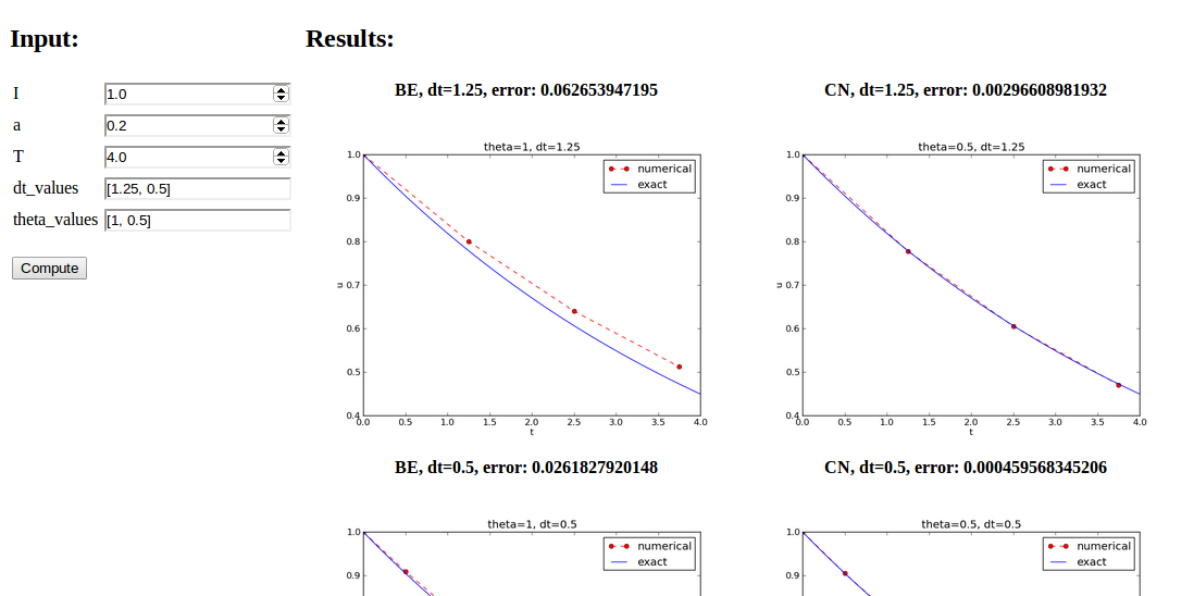
Automatically generated graphical web interface
Computing convergence rates
We expect that the error \(E\) in the numerical solution is reduced if the mesh size \(\Delta t\) is decreased. More specifically, many numerical methods obey a power-law relation between \(E\) and \(\Delta t\):
where \(C\) and \(r\) are (usually unknown) constants independent of \(\Delta t\). The formula (12) is viewed as an asymptotic model valid for sufficiently small \(\Delta t\). How small is normally hard to estimate without doing numerical estimations of \(r\).
The parameter \(r\) is known as the convergence rate. For example, if the convergence rate is 2, halving \(\Delta t\) reduces the error by a factor of 4. Diminishing \(\Delta t\) then has a greater impact on the error compared with methods that have \(r=1\). For a given value of \(r\), we refer to the method as of \(r\)-th order. First- and second-order methods are most common in scientific computing.
Estimating \(r\)
There are two alternative ways of estimating \(C\) and \(r\) based on a set of \(m\) simulations with corresponding pairs \((\Delta t_i, E_i)\), \(i=0,\ldots,m-1\), and \(\Delta t_{i} < \Delta t_{i-1}\) (i.e., decreasing cell size).
- Take the logarithm of (12), \(\ln E = r\ln \Delta t + \ln C\), and fit a straight line to the data points \((\Delta t_i, E_i)\), \(i=0,\ldots,m-1\).
- Consider two consecutive experiments, \((\Delta t_i, E_i)\) and \((\Delta t_{i-1}, E_{i-1})\). Dividing the equation \(E_{i-1}=C\Delta t_{i-1}^r\) by \(E_{i}=C\Delta t_{i}^r\) and solving for \(r\) yields
for \(i=1,\ldots,m-1\).
The disadvantage of method 1 is that (12) might not be valid for the coarsest meshes (largest \(\Delta t\) values). Fitting a line to all the data points is then misleading. Method 2 computes convergence rates for pairs of experiments and allows us to see if the sequence \(r_i\) converges to some value as \(i\rightarrow m-2\). The final \(r_{m-2}\) can then be taken as the convergence rate. If the coarsest meshes have a differing rate, the corresponding time steps are probably too large for (12) to be valid. That is, those time steps lie outside the asymptotic range of \(\Delta t\) values where the error behaves like (12).
Implementation (2)
It is straightforward to extend the main function in the program decay_argparse.py with statements for computing \(r_0, r_1, \ldots, r_{m-2}\) from (12):
from math import log

def main():
    I, a, T, makeplot, dt_values = read_command_line()
    r = {}  # estimated convergence rates
    for theta in 0, 0.5, 1:
        E_values = []
        for dt in dt_values:
            E = explore(I, a, T, dt, theta, makeplot=False)
            E_values.append(E)

        # Compute convergence rates
        m = len(dt_values)
        r[theta] = [log(E_values[i-1]/E_values[i])/
                    log(dt_values[i-1]/dt_values[i])
                    for i in range(1, m, 1)]

    for theta in r:
        print '\nPairwise convergence rates for theta=%g:' % theta
        print ' '.join(['%.2f' % r_ for r_ in r[theta]])
    return r
The program containing this main function is called decay_convrate.py.
The r object is a dictionary of lists. The keys in this dictionary are the \(\theta\) values. For example, r[1] holds the list of the \(r_i\) values corresponding to \(\theta=1\). In the loop for theta in r, the loop variable theta takes on the values of the keys in the dictionary r (in an undetermined ordering). We could simply do a print r[theta] inside the loop, but this would typically yield output of the convergence rates with 16 decimals:
[1.331919482274763, 1.1488178494691532, ...]
Instead, we format each number with 2 decimals, using a list comprehension to turn the list of numbers, r[theta], into a list of formatted strings. Then we join these strings with a space in between to get a sequence of rates on one line in the terminal window. More generally, d.join(list) joins the strings in the list list to one string, with d as delimiter between list[0], list[1], etc.
Here is an example on the outcome of the convergence rate computations:
Terminal> python decay_convrate.py --dt 0.5 0.25 0.1 0.05 0.025 0.01
...
Pairwise convergence rates for theta=0:
1.33 1.15 1.07 1.03 1.02

Pairwise convergence rates for theta=0.5:
2.14 2.07 2.03 2.01 2.01

Pairwise convergence rates for theta=1:
0.98 0.99 0.99 1.00 1.00
The Forward and Backward Euler methods seem to have an \(r\) value which stabilizes at 1, while the Crank-Nicolson seems to be a second-order method with \(r=2\).
Very often, we have some theory that predicts what \(r\) is for a numerical method. Various theoretical error measures for the \(\theta\)-rule point to \(r=2\) for \(\theta =0.5\) and \(r=1\) otherwise. The computed estimates of \(r\) are in very good agreement with these theoretical values.
Why convergence rates are important
The strong practical application of computing convergence rates is for verification: wrong convergence rates point to errors in the code, and correct convergence rates brings evidence that the implementation is correct. Experience shows that bugs in the code easily destroy the expected convergence rate.
Debugging via convergence rates
Let us experiment with bugs and see the implication on the convergence rate. We may, for instance, forget to multiply by a in the denominator in the updating formula for u[n+1]:
u[n+1] = (1 - (1-theta)*a*dt)/(1 + theta*dt)*u[n]
Running the same decay_convrate.py command as above gives the expected convergence rates (!). Why? The reason is that we just specified the \(\Delta t\) values are relied on default values for other parameters. The default value of \(a\) is 1. Forgetting the factor a has then no effect. This example shows how important it is to avoid parameters that are 1 or 0 when verifying implementations. Running the code decay_v0.py with \(a=2.1\) and \(I=0.1\) yields
Terminal> python decay_convrate.py --a 2.1 --I 0.1  \
          --dt 0.5 0.25 0.1 0.05 0.025 0.01
...
Pairwise convergence rates for theta=0:
1.49 1.18 1.07 1.04 1.02

Pairwise convergence rates for theta=0.5:
-1.42 -0.22 -0.07 -0.03 -0.01

Pairwise convergence rates for theta=1:
0.21 0.12 0.06 0.03 0.01
This time we see that the expected convergence rates for the Crank-Nicolson and Backward Euler methods are not obtained, while \(r=1\) for the Forward Euler method. The reason for correct rate in the latter case is that \(\theta=0\) and the wrong theta*dt term in the denominator vanishes anyway.
The error
u[n+1] = ((1-theta)*a*dt)/(1 + theta*dt*a)*u[n]
manifests itself through wrong rates \(r\approx 0\) for all three methods. About the same results arise from an erroneous initial condition, u[0] = 1, or wrong loop limits, range(1,Nt). It seems that in this simple problem, most bugs we can think of are detected by the convergence rate test, provided the values of the input data do not hide the bug.
A verify_convergence_rate function could compute the dictionary of list via main and check if the final rate estimates (\(r_{m-2}\)) are sufficiently close to the expected ones. A tolerance of 0.1 seems appropriate, given the uncertainty in estimating \(r\):
def verify_convergence_rate():
    r = main()
    tol = 0.1
    expected_rates = {0: 1, 1: 1, 0.5: 2}
    for theta in r:
        r_final = r[theta][-1]
        diff = abs(expected_rates[theta] - r_final)
        if diff > tol:
            return False
    return True  # all tests passed
We remark that r[theta] is a list and the last element in any list can be extracted by the index -1.
Memory-saving implementation
The computer memory requirements of our implementations so far consists mainly of the u and t arrays, both of length \(N_t+1\), plus some other temporary arrays that Python needs for intermediate results if we do array arithmetics in our program (e.g., I*exp(-a*t) needs to store a*t before - can be applied to it and then exp). The extremely modest storage requirements of simple ODE problems put no restrictions on the formulations of the algorithm and implementation. Nevertheless, when the methods for ODEs used here are applied to three-dimensional partial differential equation (PDE) problems, memory storage requirements suddenly become an issue.
The PDE counterpart to our model problem \(u'=-a\) is a diffusion equation \(u_t = a\nabla^2 u\) posed on a space-time domain. The discrete representation of this domain may in 3D be a spatial mesh of \(M^3\) points and a time mesh of \(N_t\) points. A typical desired value for \(M\) is 100 in many applications, or even \(1000\). Storing all the computed \(u\) values, like we have done in the programs so far, demands storage of some arrays of size \(M^3N_t\), giving a factor of \(M^3\) larger storage demands compared to our ODE programs. Each real number in the array for \(u\) requires 8 bytes (b) of storage. With \(M=100\) and \(N_t=1000\), there is a storage demand of \((10^3)^3\cdot 1000\cdot 8 = 8\) Gb for the solution array. Fortunately, we can usually get rid of the \(N_t\) factor, resulting in 8 Mb of storage. Below we explain how this is done, and the technique is almost always applied in implementations of PDE problems.
Let us critically evaluate how much we really need to store in the computer’s memory in our implementation of the \(\theta\) method. To compute a new \(u^{n+1}\), all we need is \(u^n\). This implies that the previous \(u^{n-1},u^{n-2},\dots,u^0\) values do not need to be stored in an array, although this is convenient for plotting and data analysis in the program. Instead of the u array we can work with two variables for real numbers, u and u_1, representing \(u^{n+1}\) and \(u^n\) in the algorithm, respectively. At each time level, we update u from u_1 and then set u_1 = u so that the computed \(u^{n+1}\) value becomes the “previous” value \(u^n\) at the next time level. The downside is that we cannot plot the solution after the simulation is done since only the last two numbers are available. The remedy is to store computed values in a file and use the file for visualizing the solution later.
We have implemented this memory saving idea in the file decay_memsave.py, which is a merge of the decay_plot_mpl.py and decay_argparse.py programs, using module prefixes np for numpy and plt for matplotlib.pyplot.
The following function demonstrates how we work with the two most recent values of the unknown:
def solver_memsave(I, a, T, dt, theta, filename='sol.dat'):
    """
    Solve u'=-a*u, u(0)=I, for t in (0,T] with steps of dt.
    Minimum use of memory. The solution is stored in a file
    (with name filename) for later plotting.
    """
    dt = float(dt)         # avoid integer division
    Nt = int(round(T/dt))  # no of intervals

    outfile = open(filename, 'w')
    # u: time level n+1, u_1: time level n
    t = 0
    u_1 = I
    outfile.write('%.16E  %.16E\n' % (t, u_1))
    for n in range(1, Nt+1):
        u = (1 - (1-theta)*a*dt)/(1 + theta*dt*a)*u_1
        u_1 = u
        t += dt
        outfile.write('%.16E  %.16E\n' % (t, u))
    outfile.close()
    return u, t
This code snippet serves as a quick introduction to file writing in Python. Reading the data in the file into arrays t and u are done by the function
def read_file(filename='sol.dat'):
    infile = open(filename, 'r')
    u = [];  t = []
    for line in infile:
        words = line.split()
        if len(words) != 2:
            print 'Found more than two numbers on a line!', words
            sys.exit(1)  # abort
        t.append(float(words[0]))
        u.append(float(words[1]))
    return np.array(t), np.array(u)
This type of file with numbers in rows and columns is very common, and numpy has a function loadtxt which loads such tabular data into a two-dimensional array, say with name data. The number in row i and column j is then data[i,j]. The whole column number j can be extracted by data[:,j]. A version of read_file using np.loadtxt reads
def read_file_numpy(filename='sol.dat'):
    data = np.loadtxt(filename)
    t = data[:,0]
    u = data[:,1]
    return t, u
The present counterpart to the explore function from decay_plot_mpl.py must run solver_memsave and then load data from file before we can compute the error measure and make the plot:
def explore(I, a, T, dt, theta=0.5, makeplot=True):
    filename = 'u.dat'
    u, t = solver_memsave(I, a, T, dt, theta, filename)

    t, u = read_file(filename)
    u_e = exact_solution(t, I, a)
    e = u_e - u
    E = np.sqrt(dt*np.sum(e**2))
    if makeplot:
        plt.figure()
        ...
The decay_memsave.py file also includes command-line options --I, --a, --T, --dt, --theta, and --makeplot for controlling input parameters and making a single run. For example,
Terminal> python decay_memsave.py --T 10 --theta 1 --dt 2
results in the output
I=1.0, a=1.0, T=10.0, makeplot=True, theta=1.0, dt=2.0
theta=1.0 dt=2 Error=3.136E-01
![]()
Table Of Contents
- Implementation (1)
