Finite difference methods

Goal

We explain the basic ideas of finite difference methods using a simple ordinary differential equation \(u'=-au\) as primary example. Emphasis is put on the reasoning when discretizing the problem and introduction of key concepts such as mesh, mesh function, finite difference approximations, averaging in a mesh, deriation of algorithms, and discrete operator notation.

A basic model for exponential decay

Our model problem is perhaps the simplest ordinary differential equation (ODE):

\[u'(t) = -au(t),\]

Here, \(a>0\) is a constant and \(u'(t)\) means differentiation with respect to time \(t\). This type of equation arises in a number of widely different phenomena where some quantity \(u\) undergoes exponential reduction. Examples include radioactive decay, population decay, investment decay, cooling of an object, pressure decay in the atmosphere, and retarded motion in fluids (for some of these models, \(a\) can be negative as well), see the section Applications of exponential decay models for details and motivation. We have chosen this particular ODE not only because its applications are relevant, but even more because studying numerical solution methods for this simple ODE gives important insight that can be reused in much more complicated settings, in particular when solving diffusion-type partial differential equations.

The analytical solution of the ODE is found by the method of separation of variables, which results in

\[u(t) = Ce^{-at},\]

for any arbitrary constant \(C\). To formulate a mathematical problem for which there is a unique solution, we need a condition to fix the value of \(C\). This condition is known as the initial condition and stated as \(u(0)=I\). That is, we know the value \(I\) of \(u\) when the process starts at \(t=0\). The exact solution is then \(u(t)=Ie^{-at}\).

We seek the solution \(u(t)\) of the ODE for \(t\in (0,T]\). The point \(t=0\) is not included since we know \(u\) here and assume that the equation governs \(u\) for \(t>0\). The complete ODE problem then reads: find \(u(t)\) such that

(1)\[ u' = -au,\ t\in (0,T], \quad u(0)=I{\thinspace .}\]

This is known as a continuous problem because the parameter \(t\) varies continuously from \(0\) to \(T\). For each \(t\) we have a corresponding \(u(t)\). There are hence infinitely many values of \(t\) and \(u(t)\). The purpose of a numerical method is to formulate a corresponding discrete problem whose solution is characterized by a finite number of values, which can be computed in a finite number of steps on a computer.

The Forward Euler scheme

Solving an ODE like (1) by a finite difference method consists of the following four steps:

1. discretizing the domain,
2. fulfilling the equation at discrete time points,
3. replacing derivatives by finite differences,
4. formulating a recursive algorithm.

Step 1: Discretizing the domain

The time domain \([0,T]\) is represented by a finite number of \(N_t+1\) points

\[\begin{split}0 = t_0 < t_1 < t_2 < \cdots < t_{N_t-1} < t_{N_t} = T{\thinspace .}\end{split}\]

The collection of points \(t_0,t_1,\ldots,t_{N_t}\) constitutes a mesh or grid. Often the mesh points will be uniformly spaced in the domain \([0,T]\), which means that the spacing \(t_{n+1}-t_n\) is the same for all \(n\). This spacing is often denoted by \(\Delta t\), in this case \(t_n=n\Delta t\).

We seek the solution \(u\) at the mesh points: \(u(t_n)\), \(n=1,2,\ldots,N_t\). Note that \(u^0\) is already known as \(I\). A notational short-form for \(u(t_n)\), which will be used extensively, is \(u^{n}\). More precisely, we let \(u^n\) be the numerical approximation to the exact solution \(u(t_n)\) at \(t=t_n\). The numerical approximation is a mesh function, here defined only at the mesh points. When we need to clearly distinguish between the numerical and the exact solution, we often place a subscript e on the exact solution, as in \({u_{\small\mbox{e}}}(t_n)\). Figure Time mesh with discrete solution values shows the \(t_n\) and \(u_n\) points for \(n=0,1,\ldots,N_t=7\) as well as \({u_{\small\mbox{e}}}(t)\) as the dashed line. The goal of a numerical method for ODEs is to compute the mesh function by solving a finite set of algebraic equations derived from the original ODE problem.

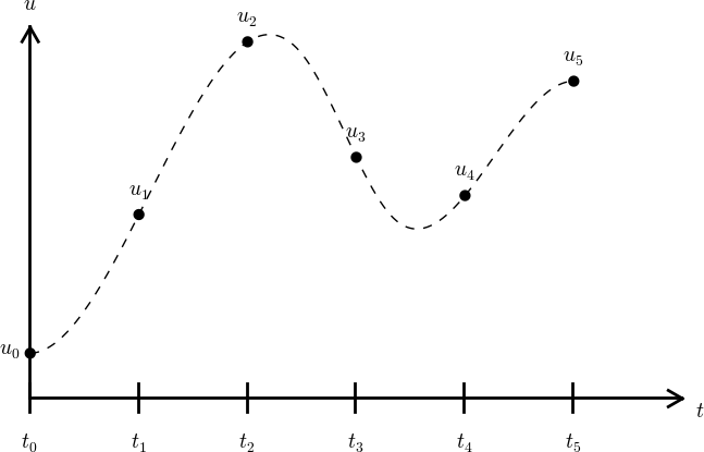
Time mesh with discrete solution values

Since finite difference methods produce solutions at the mesh points only, it is an open question what the solution is between the mesh points. One can use methods for interpolation to compute the value of \(u\) between mesh points. The simplest (and most widely used) interpolation method is to assume that \(u\) varies linearly between the mesh points, see Figure Linear interpolation between the discrete solution values (dashed curve is exact solution). Given \(u^{n}\) and \(u^{n+1}\), the value of \(u\) at some \(t\in [t_{n}, t_{n+1}]\) is by linear interpolation

\[u(t) \approx u^n + \frac{u^{n+1}-u^n}{t_{n+1}-t_n}(t - t_n){\thinspace .}\]

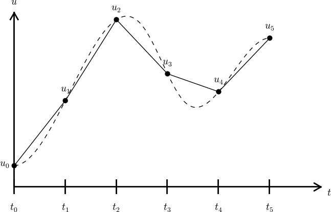
Linear interpolation between the discrete solution values (dashed curve is exact solution)

Step 2: Fulfilling the equation at discrete time points

The ODE is supposed to hold for all \(t\in (0,T]\), i.e., at an infinite number of points. Now we relax that requirement and require that the ODE is fulfilled at a finite set of discrete points in time. The mesh points \(t_1,t_2,\ldots,t_{N_t}\) are a natural choice of points. The original ODE is then reduced to the following \(N_t\) equations:

(2)\[ u'(t_n) = -au(t_n),\quad n=1,\ldots,N_t{\thinspace .}\]

Step 3: Replacing derivatives by finite differences

The next and most essential step of the method is to replace the derivative \(u'\) by a finite difference approximation. Let us first try a one-sided difference approximation (see Figure Illustration of a forward difference),

(3)\[ u'(t_n) \approx \frac{u^{n+1}-u^{n}}{t_{n+1}-t_n}{\thinspace .}\]

Inserting this approximation in (2) results in

(4)\[ \frac{u^{n+1}-u^{n}}{t_{n+1}-t_n} = -au^{n},\quad n=0,1,\ldots,N_t-1{\thinspace .}\]

This equation is the discrete counterpart to the original ODE problem (1), and often referred to as finite difference scheme or more generally as the discrete equations of the problem. The fundamental feature of these equations is that they are algebraic and can hence be straightforwardly solved to produce the mesh function, i.e., the values of \(u\) at the mesh points (\(u^n\), \(n=1,2,\ldots,N_t\)).

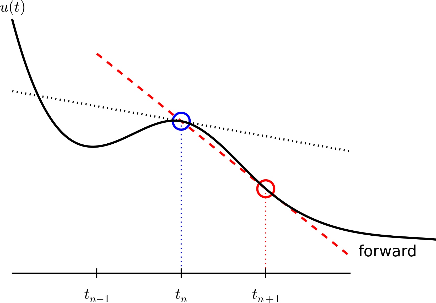
Illustration of a forward difference

Step 4: Formulating a recursive algorithm

The final step is to identify the computational algorithm to be implemented in a program. The key observation here is to realize that (4) can be used to compute \(u^{n+1}\) if \(u^n\) is known. Starting with \(n=0\), \(u^0\) is known since \(u^0=u(0)=I\), and (4) gives an equation for \(u^1\). Knowing \(u^1\), \(u^2\) can be found from (4). In general, \(u^n\) in (4) can be assumed known, and then we can easily solve for the unknown \(u^{n+1}\):

(5)\[ u^{n+1} = u^n - a(t_{n+1} -t_n)u^n{\thinspace .}\]

We shall refer to (5) as the Forward Euler (FE) scheme for our model problem. From a mathematical point of view, equations of the form (5) are known as difference equations since they express how differences in \(u\), like \(u^{n+1}-u^n\), evolve with \(n\). The finite difference method can be viewed as a method for turning a differential equation into a difference equation.

Computation with (5) is straightforward:

\[\begin{split}u_0 &= I,\\ u_1 & = u^0 - a(t_{1} -t_0)u^0 = I(1-a(t_1-t_0)),\\ u_2 & = u^1 - a(t_{2} -t_1)u^1 = I(1-a(t_1-t_0))(1 - a(t_2-t_1)),\\ u^3 &= u^2 - a(t_{3} -t_2)u^2 = I(1-a(t_1-t_0))(1 - a(t_2-t_1))(1 - a(t_3-t_2)),\end{split}\]

and so on until we reach \(u^{N_t}\). Very often, \(t_{n+1}-t_n\) is constant for all \(n\), so we can introduce the common symbol \(\Delta t\) for the time step: \(\Delta t = t_{n+1}-t_n\), \(n=0,1,\ldots,N_t-1\). Using a constant time step \(\Delta t\) in the above calculations gives

\[\begin{split}u_0 &= I,\\ u_1 & = I(1-a\Delta t),\\ u_2 & = I(1-a\Delta t)^2,\\ u^3 &= I(1-a\Delta t)^3,\\ &\vdots\\ u^{N_t} &= I(1-a\Delta t)^{N_t}{\thinspace .}\end{split}\]

This means that we have found a closed formula for \(u^n\), and there is no need to let a computer generate the sequence \(u^1, u^2, u^3, \ldots\). However, finding such a formula for \(u^n\) is possible only for a few very simple problems, so in general finite difference equations must be solved on a computer.

As the next sections will show, the scheme (5) is just one out of many alternative finite difference (and other) methods for the model problem (1).

The Backward Euler scheme

There are several choices of difference approximations in step 3 of the finite difference method as presented in the previous section. Another alternative is

(6)\[ u'(t_n) \approx \frac{u^{n}-u^{n-1}}{t_{n}-t_{n-1}}{\thinspace .}\]

Since this difference is based on going backward in time (\(t_{n-1}\)) for information, it is known as the Backward Euler difference. Figure Illustration of a backward difference explains the idea.

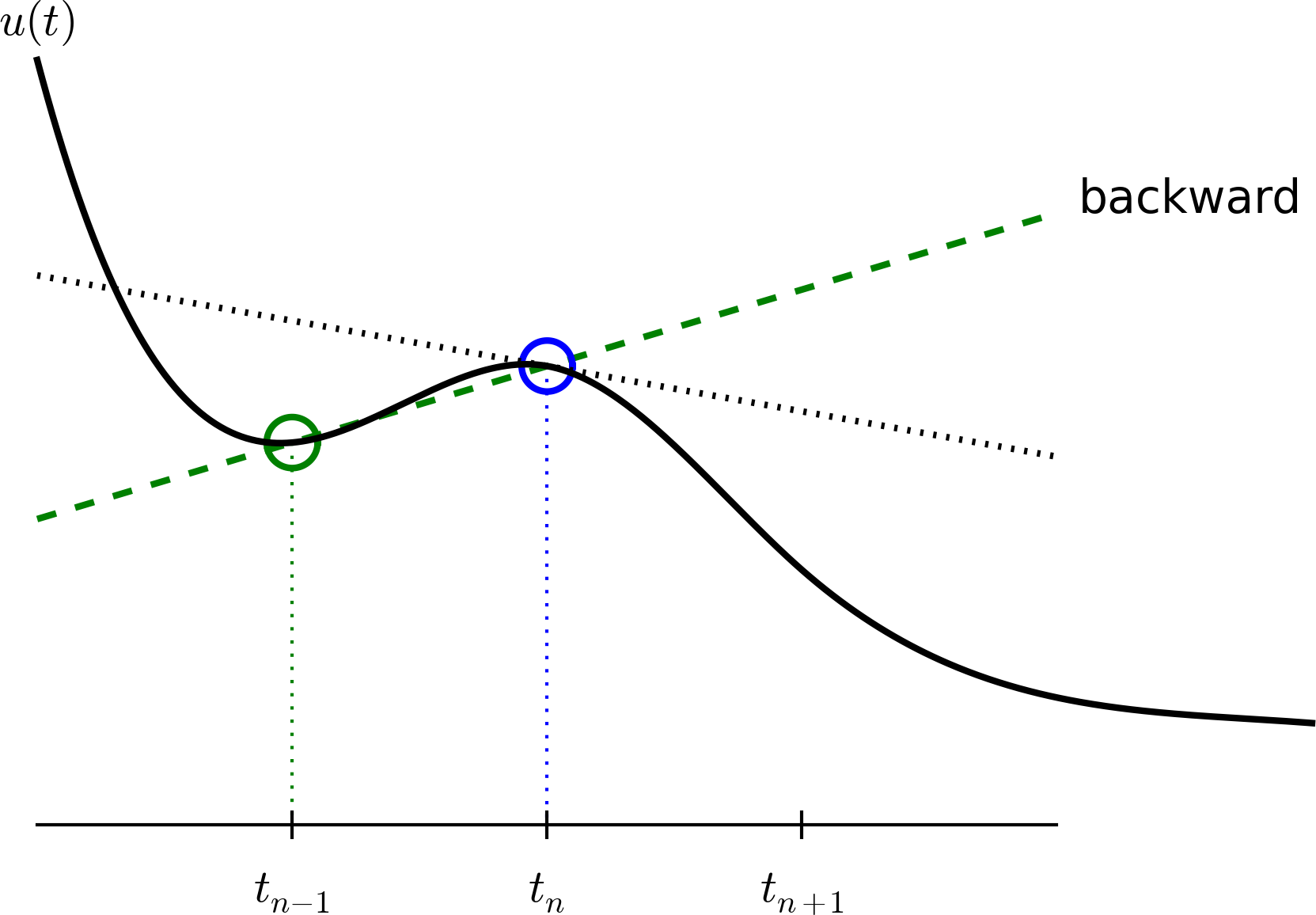
Illustration of a backward difference

Inserting (6) in (2) yields the Backward Euler (BE) scheme:

(7)\[ \frac{u^{n}-u^{n-1}}{t_{n}-t_{n-1}} = -a u^n{\thinspace .}\]

We assume, as explained under step 4 in the section The Forward Euler scheme, that we have computed \(u^0, u^1, \ldots, u^{n-1}\) such that (7) can be used to compute \(u^n\). For direct similarity with the Forward Euler scheme (5) we replace \(n\) by \(n+1\) in (7) and solve for the unknown value \(u^{n+1}\):

(8)\[ u^{n+1} = \frac{1}{1+ a(t_{n+1}-t_n)} u^n{\thinspace .}\]

The Crank-Nicolson scheme

The finite difference approximations used to derive the schemes (5) and (8) are both one-sided differences, known to be less accurate than central (or midpoint) differences. We shall now construct a central difference at \(t_{n+1/2}=\frac{1}{2} (t_n + t_{n+1})\), or \(t_{n+1/2}=(n+\frac{1}{2})\Delta t\) if the mesh spacing is uniform in time. The approximation reads

(9)\[ u'(t_{n+\frac{1}{2}}) \approx \frac{u^{n+1}-u^n}{t_{n+1}-t_n}{\thinspace .}\]

Note that the fraction on the right-hand side is the same as for the Forward Euler approximation (3) and the Backward Euler approximation (6) (with \(n\) replaced by \(n+1\)). The accuracy of this fraction as an approximation to the derivative of \(u\) depends on where we seek the derivative: in the center of the interval \([t_{n},t_{n+1}]\) or at the end points.

With the formula (9), where \(u'\) is evaluated at \(t_{n+1/2}\), it is natural to demand the ODE to be fulfilled at the time points between the mesh points:

(10)\[ u'(t_{n+\frac{1}{2}}) = -au(t_{n+\frac{1}{2}}),\quad n=0, \ldots,N_t-1{\thinspace .}\]

Using (9) in (10) results in

(11)\[ \frac{u^{n+1}-u^n}{t_{n+1}-t_n} = -au^{n+\frac{1}{2}},\]

where \(u^{n+\frac{1}{2}}\) is a short form for \(u(t_{n+\frac{1}{2}})\). The problem is that we aim to compute \(u^n\) for integer \(n\), implying that \(u^{n+\frac{1}{2}}\) is not a quantity computed by our method. It must therefore be expressed by the quantities that we actually produce, i.e., the numerical solution at the mesh points. One possibility is to approximate \(u^{n+\frac{1}{2}}\) as an arithmetic mean of the \(u\) values at the neighboring mesh points:

(12)\[ u^{n+\frac{1}{2}} \approx \frac{1}{2} (u^n + u^{n+1}){\thinspace .}\]

Using (12) in (11) results in

(13)\[ \frac{u^{n+1}-u^n}{t_{n+1}-t_n} = -a\frac{1}{2} (u^n + u^{n+1}){\thinspace .}\]

Figure Illustration of a centered difference sketches the geometric interpretation of such a centered difference.

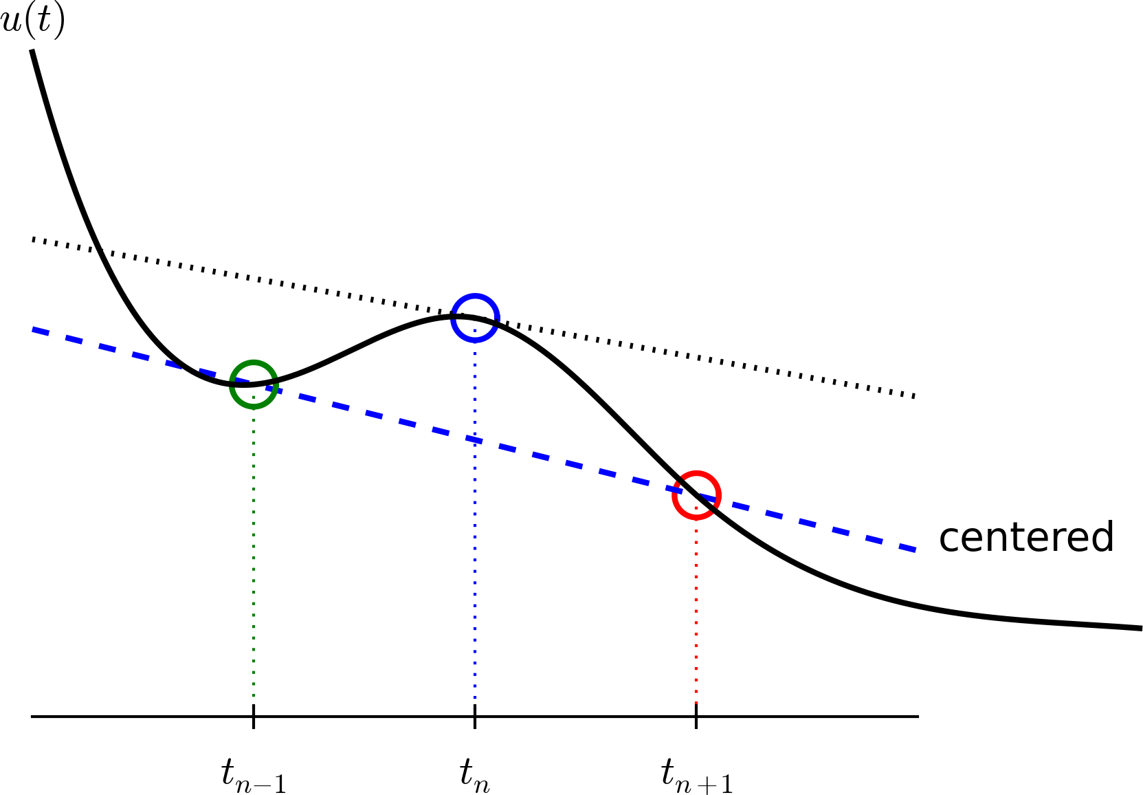
Illustration of a centered difference

We assume that \(u^n\) is already computed so that \(u^{n+1}\) is the unknown, which we can solve for:

(14)\[ u^{n+1} = \frac{1-\frac{1}{2} a(t_{n+1}-t_n)}{1 + \frac{1}{2} a(t_{n+1}-t_n)}u^n{\thinspace .}\]

The finite difference scheme (14) is often called the Crank-Nicolson (CN) scheme or a midpoint or centered scheme.

The unifying \(\theta\)-rule

The Forward Euler, Backward Euler, and Crank-Nicolson schemes can be formulated as one scheme with a varying parameter \(\theta\):

(15)\[ \frac{u^{n+1}-u^{n}}{t_{n+1}-t_n} = -a (\theta u^{n+1} + (1-\theta) u^{n})\]\[ {\thinspace .}\]

Observe:

• \(\theta =0\) gives the Forward Euler scheme
• \(\theta =1\) gives the Backward Euler scheme, and
• \(\theta =\frac{1}{2}\) gives the Crank-Nicolson scheme.
• We may alternatively choose any other value of \(\theta\) in \([0,1]\).

As before, \(u^n\) is considered known and \(u^{n+1}\) unknown, so we solve for the latter:

(16)\[ u^{n+1} = \frac{1 - (1-\theta) a(t_{n+1}-t_n)}{1 + \theta a(t_{n+1}-t_n)}{\thinspace .}\]

This scheme is known as the \(\theta\)-rule, or alternatively written as the “theta-rule”.

Derivation

We start with replacing \(u'\) by the fraction

\[\frac{u^{n+1}-u^{n}}{t_{n+1}-t_n},\]

in the Forward Euler, Backward Euler, and Crank-Nicolson schemes. Then we observe that the difference between the methods concerns which point this fraction approximates the derivative. Or in other words, at which point we sample the ODE. So far this has been the end points or the midpoint of \([t_n,t_{n+1}]\). However, we may choose any point \(\tilde t \in [t_n,t_{n+1}]\). The difficulty is that evaluating the right-hand side \(-au\) at an arbitrary point faces the same problem as in the section The Crank-Nicolson scheme: the point value must be expressed by the discrete \(u\) quantities that we compute by the scheme, i.e., \(u^n\) and \(u^{n+1}\). Following the averaging idea from the section The Crank-Nicolson scheme, the value of \(u\) at an arbitrary point \(\tilde t\) can be calculated as a weighted average, which generalizes the arithmetic mean \(\frac{1}{2} u^n + {\frac{1}{2}}u^{n+1}\). If we express \(\tilde t\) as a weighted average

\[t_{n+\theta} = \theta t_{n+1} + (1-\theta) t_{n},\]

where \(\theta\in [0,1]\) is the weighting factor, we can write

(17)\[ u(\tilde t) = u(\theta t_{n+1} + (1-\theta) t_{n}) \approx \theta u^{n+1} + (1-\theta) u^{n}{\thinspace .}\]\[.. index:: theta-rule\]\[ We can now let the ODE hold at the point :math:`\tilde t\in [t_n,t_{n+1}]`, approximate :math:`u'` by the fraction :math:`(u^{n+1}-u^{n})/(t_{n+1}-t_n)`, and approximate the right-hand side :math:`-au` by the weighted average :eq:`decay:thetaavg`. The result is :eq:`decay:th0`.\]

Constant time step

All schemes up to now have been formulated for a general non-uniform mesh in time: \(t_0,t_1,\ldots,t_{N_t}\). Non-uniform meshes are highly relevant since one can use many points in regions where \(u\) varies rapidly, and save points in regions where \(u\) is slowly varying. This is the key idea of adaptive methods where the spacing of the mesh points are determined as the computations proceed.

However, a uniformly distributed set of mesh points is very common and sufficient for many applications. It therefore makes sense to present the finite difference schemes for a uniform point distribution \(t_n=n\Delta t\), where \(\Delta t\) is the constant spacing between the mesh points, also referred to as the time step. The resulting formulas look simpler and are perhaps more well known.

Summary of schemes for constant time step

(18)\[ u^{n+1} = (1 - a\Delta t )u^n \quad (\hbox{FE})\]\[.. _Eq:decay:BE:u:\]

(19)\[ u^{n+1} = \frac{1}{1+ a\Delta t} u^n \quad (\hbox{BE})\]\[.. _Eq:decay:CN:u:\]

(20)\[ u^{n+1} = \frac{1-\frac{1}{2} a\Delta t}{1 + \frac{1}{2} a\Delta t} u^n \quad (\hbox{CN})\]\[.. _Eq:decay:th:u:\]

(21)\[ u^{n+1} = \frac{1 - (1-\theta) a\Delta t}{1 + \theta a\Delta t}u^n \quad (\theta-\hbox{rule})\]

Not surprisingly, we present these three alternative schemes because they have different pros and cons, both for the simple ODE in question (which can easily be solved as accurately as desired), and for more advanced differential equation problems.

Test the understanding

At this point it can be good training to apply the explained finite difference discretization techniques to a slightly different equation. Exercise 1: Derive schemes for Newton’s law of cooling is therefore highly recommended to check that the key concepts are understood.

Compact operator notation for finite differences

Finite difference formulas can be tedious to write and read, especially for differential equations with many terms and many derivatives. To save space and help the reader of the scheme to quickly see the nature of the difference approximations, we introduce a compact notation. A forward difference approximation is denoted by the \(D_t^+\) operator:

(22)\[ [D_t^+u]^n = \frac{u^{n+1} - u^{n}}{\Delta t} \approx \frac{d}{dt} u(t_n) {\thinspace .}\]

The notation consists of an operator that approximates differentiation with respect to an independent variable, here \(t\). The operator is built of the symbol \(D\), with the variable as subscript and a superscript denoting the type of difference. The superscript \(\,{}^+\) indicates a forward difference. We place square brackets around the operator and the function it operates on and specify the mesh point, where the operator is acting, by a superscript.

The corresponding operator notation for a centered difference and a backward difference reads

(23)\[ [D_tu]^n = \frac{u^{n+\frac{1}{2}} - u^{n-\frac{1}{2}}}{\Delta t} \approx \frac{d}{dt} u(t_n),\]

and

(24)\[ [D_t^-u]^n = \frac{u^{n} - u^{n-1}}{\Delta t} \approx \frac{d}{dt} u(t_n) {\thinspace .}\]

Note that the superscript \(\,{}^-\) denotes the backward difference, while no superscript implies a central difference.

An averaging operator is also convenient to have:

(25)\[ [\overline{u}^{t}]^n = \frac{1}{2} (u^{n-\frac{1}{2}} + u^{n+\frac{1}{2}} ) \approx u(t_n)\]

The superscript \(t\) indicates that the average is taken along the time coordinate. The common average \((u^n + u^{n+1})/2\) can now be expressed as \([\overline{u}^{t}]^{n+\frac{1}{2}}\). (When also spatial coordinates enter the problem, we need the explicit specification of the coordinate after the bar.)

The Backward Euler finite difference approximation to \(u'=-au\) can be written as follows utilizing the compact notation:

\[[D_t^-u]^n = -au^n {\thinspace .}\]

In difference equations we often place the square brackets around the whole equation, to indicate at which mesh point the equation applies, since each term is supposed to be approximated at the same point:

\[[D_t^- u = -au]^n {\thinspace .}\]

The Forward Euler scheme takes the form

\[[D_t^+ u = -au]^n,\]

while the Crank-Nicolson scheme is written as

(26)\[ [D_t u = -a\overline{u}^t]^{n+\frac{1}{2}}{\thinspace .}\]

Question

Apply (23) and (25) and write out the expressions to see that (26) is indeed the Crank-Nicolson scheme.

The \(\theta\)-rule can be specified by

(27)\[ [\bar D_t u = -a\overline{u}^{t,\theta}]^{n+\theta},\]

if we define a new time difference and a weighted averaging operator:

\[\lbrack\bar D_t u\rbrack^{n+\theta} = \frac{u^{n+1}-u^n}{t^{n+1}-t^n},\]\[\lbrack\overline{u}^{t,\theta}\rbrack^{n+\theta} = (1-\theta)u^{n} + \theta u^{n+1} \approx u(t_{n+\theta}),\]

where \(\theta\in [0,1]\). Note that for \(\theta =\frac{1}{2}\) we recover the standard centered difference and the standard arithmetic mean. The idea in (27) is to sample the equation at \(t_{n+\theta}\), use a skew difference at that point \([\bar D_t u]^{n+\theta}\), and a skew mean value. An alternative notation is

\[[D_t u]^{n+\frac{1}{2}} = \theta [-au]^{n+1} + (1-\theta)[-au]^{n}{\thinspace .}\]

Looking at the various examples above and comparing them with the underlying differential equations, we see immediately which difference approximations that have been used and at which point they apply. Therefore, the compact notation effectively communicates the reasoning behind turning a differential equation into a difference equation.