$$
\newcommand{\uex}{{u_{\small\mbox{e}}}}
\newcommand{\half}{\frac{1}{2}}
\newcommand{\halfi}{{1/2}}
\newcommand{\xpoint}{\boldsymbol{x}}
\newcommand{\normalvec}{\boldsymbol{n}}
\newcommand{\Oof}[1]{\mathcal{O}(#1)}
\newcommand{\Ix}{\mathcal{I}_x}
\newcommand{\Iy}{\mathcal{I}_y}
\newcommand{\It}{\mathcal{I}_t}
\newcommand{\setb}[1]{#1^0} % set begin
\newcommand{\sete}[1]{#1^{-1}} % set end
\newcommand{\setl}[1]{#1^-}
\newcommand{\setr}[1]{#1^+}
\newcommand{\seti}[1]{#1^i}
\newcommand{\Real}{\mathbb{R}}
$$
The discrete solution
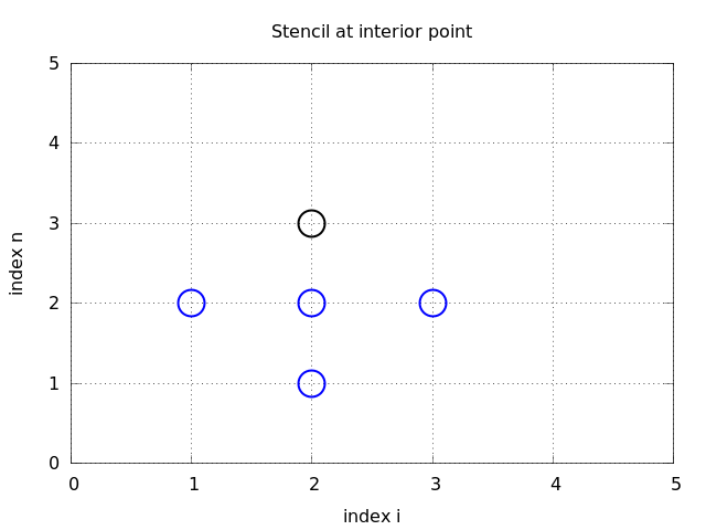
- The numerical solution is a mesh function: \( u_i^n \approx \uex(x_i,t_n) \)
- Finite difference stencil (or scheme): equation for \( u^n_i \) involving
neighboring space-time points