Goal
This document illustrates best practice for developing scientific software in an efficient and reliable way. Not only will the outlined techniques save a lost of human time, but they will also help assure reproducible science and higher quality of computational investigations. Key questions to be answered are
- How should I organize a program?
- How can I efficiently and safely provide input data and run my code?
- How can I verify that the implementation is correct?
- How should I reliably work with files and documents?
- How should I conduct large numerical experiments?
Sample problem and code
This first introduction to good programming habits in scientific computing will make use of a very simple mathematical problem to keep the mathematical details at the lowest possible level while introducing a series of computer science concepts. The simplicity of the mathematical problem obviously prevents us from treating several techniques that are only meaningful for complex scientific software.
Mathematical problem
We consider the simplest possible ordinary differential equation with constant coefficient \(a\):
This problem is numerically solved by the so-called \(\theta\)-rule, which is a convenient way to merge different formulas for the well-known Forward Euler, Backward Euler, and Crank-Nicolson (midpoint/central) schemes. We introduce a uniform time mesh \(t_n=n\Delta t\), \(n=0,1,\ldots,N_t\), and seek \(u(t)\) at the mesh points. The numerical approximation to \(u(t_n)\) is denoted \(u^n\). Since we will use the symbol \(u\) both for the exact analytical solution of (1) and for the numerical approximation, we sometimes introduce \({u_{\small\mbox{e}}}(t)\) to help distinguish the two types of solutions (i.e., subscript e for “exact”) [1].
| [1] | In the literature, it is more common to put a subscript (like \(u_\Delta\) or \(u_h\)) on the numerical solution to distinguish it from the exact solution. However, we will use the variable u in the code for the numerical approximation to be computed, and therefore adjust the mathematical notation to convenient conventions in the code such that we can have as close correspondence as possible between the implementation and the mathematics. |
The \(\theta\)-rule leads to an explicit updating formula for \(u^{n+1}\), given \(u^n\):
Implementation (1)
The numerical method is implemented as a function solver. Another function explore computes the error in the solution, by comparing with the exact solution \({u_{\small\mbox{e}}}(t)=Ie^{-at}\), and creates a plot for comparing the numerical and exact solution.
The program file decay_plot.py contains the two functions and a main program.
from numpy import *
from matplotlib.pyplot import *

def solver(I, a, T, dt, theta):
    """Solve u'=-a*u, u(0)=I, for t in (0,T] with steps of dt."""
    dt = float(dt)            # avoid integer division
    Nt = int(round(T/dt))     # no of time intervals
    T = Nt*dt                 # adjust T to fit time step dt
    u = zeros(Nt+1)           # array of u[n] values
    t = linspace(0, T, Nt+1)  # time mesh

    u[0] = I                  # assign initial condition
    for n in range(0, Nt):    # n=0,1,...,Nt-1
        u[n+1] = (1 - (1-theta)*a*dt)/(1 + theta*dt*a)*u[n]
    return u, t

def exact_solution(t, I, a):
    return I*exp(-a*t)

def explore(I, a, T, dt, theta=0.5, makeplot=True):
    """
    Run a case with the solver, compute error measure,
    and plot the numerical and exact solutions (if makeplot=True).
    """
    u, t = solver(I, a, T, dt, theta)    # Numerical solution
    u_e = exact_solution(t, I, a)
    e = u_e - u
    E = sqrt(dt*sum(e**2))
    if makeplot:
        figure()                         # create new plot
        t_e = linspace(0, T, 1001)       # fine mesh for u_e
        u_e = exact_solution(t_e, I, a)
        plot(t,   u,   'r--o')           # red dashes w/circles
        plot(t_e, u_e, 'b-')             # blue line for exact sol.
        legend(['numerical', 'exact'])
        xlabel('t')
        ylabel('u')
        title('theta=%g, dt=%g' % (theta, dt))
        theta2name = {0: 'FE', 1: 'BE', 0.5: 'CN'}
        savefig('%s_%g.png' % (theta2name[theta], dt))
        savefig('%s_%g.pdf' % (theta2name[theta], dt))
        show()
    return E

def main(I, a, T, dt_values, theta_values=(0, 0.5, 1)):
    for theta in theta_values:
        for dt in dt_values:
            E = explore(I, a, T, dt, theta, makeplot=True)
            print '%3.1f %6.2f: %12.3E' % (theta, dt, E)

main(I=1, a=2, T=5, dt_values=[0.4, 0.04])
User interfaces
It is good programming practice to let programs read input from the user rather than require the user to edit the source code when trying out new values of input parameters. One reason is that any edit of the code has a danger of introducing bugs. Another reason is that it is easier and less manual work to supply data to a program instead of editing the program code. A third reason is that a program that reads input can easily be run by another program, and in this way we can automate a large number of runs in scientific investigations.
Tip
We shall make it a habit to equip any implementation of a numerical solver with an appropriate user interface before testing out the code.
Reading input data can be done in many ways. We have to decide on desired user interface, i.e., how we want to operate the program when providing input, and then use appropriate tools to implement the user interface. There are four basic types of user interface of relevance to our programs, listed here with increasing complexity of the implementation:
- Questions and answers in the terminal window
- Command-line arguments
- Reading data from file
- Graphical user interfaces
Although conceptually simple, alternative 1 involves more typing than the other alternatives and is therefore abandoned. Below, we shall address alternative 2 and 4, which are most appropriate for the present problem.
[[[ .. _decay:commandline:
Creating command-line interfaces
Reading input from the command line is a simple and flexible way of interacting with the user. Python stores all the command-line arguments in the list sys.argv, and there are, in principle, two ways of programming with command-line arguments in Python:
- Decide upon a sequence of parameters on the command line and read their values directly from the sys.argv[1:] list (sys.argv[0] is the just program name).
- Use option-value pairs (--option value) on the command line to override default values of input parameters, and utilize the argparse.ArgumentParser tool to interact with the command line.
Both strategies will be illustrated next.
Reading a sequence of command-line arguments
The decay_plot.py program needs the following input data: \(I\), \(a\), \(T\), an option to turn the plot on or off (makeplot), and a list of \(\Delta t\) values.
The simplest way of reading this input from the command line is to say that the first four command-line arguments correspond to the first four points in the list above, in that order, and that the rest of the command-line arguments are the \(\Delta t\) values. The input given for makeplot can be a string among 'on', 'off', 'True', and 'False'. The code for reading this input is most conveniently put in a function:
import sys

def read_command_line():
    if len(sys.argv) < 6:
        print 'Usage: %s I a T on/off dt1 dt2 dt3 ...' % \
              sys.argv[0]; sys.exit(1)  # abort

    I = float(sys.argv[1])
    a = float(sys.argv[2])
    T = float(sys.argv[3])
    makeplot = sys.argv[4] in ('on', 'True')
    dt_values = [float(arg) for arg in sys.argv[5:]]

    return I, a, T, makeplot, dt_values
One should note the following about the constructions in the program above:
- Everything on the command line ends up in a string in the list sys.argv. Explicit conversion to, e.g., a float object is required if the string as a number we want to compute with.
- The value of makeplot is determined from a boolean expression, which becomes True if the command-line argument is either 'on' or 'True', and False otherwise.
- It is easy to build the list of \(\Delta t\) values: we simply run through the rest of the list, sys.argv[5:], convert each command-line argument to float, and collect these float objects in a list, using the compact and convenient list comprehension syntax in Python.
The loops over \(\theta\) and \(\Delta t\) values can be coded in a main function:
def main():
    I, a, T, makeplot, dt_values = read_command_line()
    for theta in 0, 0.5, 1:
        for dt in dt_values:
            E = explore(I, a, T, dt, theta, makeplot)
            print '%3.1f %6.2f: %12.3E' % (theta, dt, E)
The complete program can be found in decay_cml.py.
Working with an argument parser
Python’s ArgumentParser tool in the argparse module makes it easy to create a professional command-line interface to any program. The documentation of ArgumentParser demonstrates its versatile applications, so we shall here just list an example containing basic features. On the command line we want to specify option-value pairs for \(I\), \(a\), and \(T\), e.g., --a 3.5 --I 2 --T 2. Including --makeplot turns the plot on and excluding this option turns the plot off. The \(\Delta t\) values can be given as --dt 1 0.5 0.25 0.1 0.01. Each parameter must have a sensible default value so that we specify the option on the command line only when the default value is not suitable.
We introduce a function for defining the mentioned command-line options:
def define_command_line_options():
    import argparse
    parser = argparse.ArgumentParser()
    parser.add_argument('--I', '--initial_condition', type=float,
                        default=1.0, help='initial condition, u(0)',
                        metavar='I')
    parser.add_argument('--a', type=float,
                        default=1.0, help='coefficient in ODE',
                        metavar='a')
    parser.add_argument('--T', '--stop_time', type=float,
                        default=1.0, help='end time of simulation',
                        metavar='T')
    parser.add_argument('--makeplot', action='store_true',
                        help='display plot or not')
    parser.add_argument('--dt', '--time_step_values', type=float,
                        default=[1.0], help='time step values',
                        metavar='dt', nargs='+', dest='dt_values')
    return parser
Each command-line option is defined through the parser.add_argument method. Alternative options, like the short --I and the more explaining version --initial_condition can be defined. Other arguments are type for the Python object type, a default value, and a help string, which gets printed if the command-line argument -h or --help is included. The metavar argument specifies the value associated with the option when the help string is printed. For example, the option for \(I\) has this help output:
Terminal> python decay_argparse.py -h
  ...
  --I I, --initial_condition I
                        initial condition, u(0)
  ...
The structure of this output is
--I metavar, --initial_condition metavar
                      help-string
The --makeplot option is a pure flag without any value, implying a true value if the flag is present and otherwise a false value. The action='store_true' makes an option for such a flag.
Finally, the --dt option demonstrates how to allow for more than one value (separated by blanks) through the nargs='+' keyword argument. After the command line is parsed, we get an object where the values of the options are stored as attributes. The attribute name is specified by the dist keyword argument, which for the --dt option is dt_values. Without the dest argument, the value of an option --opt is stored as the attribute opt.
The code below demonstrates how to read the command line and extract the values for each option:
def read_command_line():
    parser = define_command_line_options()
    args = parser.parse_args()
    print 'I={}, a={}, T={}, makeplot={}, dt_values={}'.format(
        args.I, args.a, args.T, args.makeplot, args.dt_values)
    return args.I, args.a, args.T, args.makeplot, args.dt_values
The main function remains the same as in the decay_cml.py code based on reading from sys.argv directly. A complete program featuring the demo above of ArgumentParser appears in the file decay_argparse.py.
Creating a graphical web user interface
The Python package Parampool can be used to automatically generate a web-based graphical user interface (GUI) for our simulation program. Although the programming technique dramatically simplifies the efforts to create a GUI, the forthcoming material on equipping our decay_mod module with a GUI is quite technical and of significantly less importance than knowing how to make a command-line interface (the section decay:commandline). There is no danger in jumping right to the section Computing convergence rates.
Making a compute function
The first step is to identify a function that performs the computations and that takes the necessary input variables as arguments. This is called the compute function in Parampool terminology. We may start with a copy of the basic file decay_plot.py, which has a main function displayed in the section decay:plotting for carrying out simulations and plotting for a series of \(\Delta t\) values. Now we want to control and view the same experiments from a web GUI.
To tell Parampool what type of input data we have, we assign default values of the right type to all arguments in the main function and call it main_GUI:
def main_GUI(I=1.0, a=.2, T=4.0,
         dt_values=[1.25, 0.75, 0.5, 0.1],
         theta_values=[0, 0.5, 1]):
The compute function must return the HTML code we want for displaying the result in a web page. Here we want to show plots of the numerical and exact solution for different methods and \(\Delta t\) values. The plots can be organized in a table with \(\theta\) (methods) varying through the columns and \(\Delta t\) varying through the rows. Assume now that a new version of the explore function not only returns the error E but also HTML code containing the plot. Then we can write the main_GUI function as
def main_GUI(I=1.0, a=.2, T=4.0,
         dt_values=[1.25, 0.75, 0.5, 0.1],
         theta_values=[0, 0.5, 1]):
    # Build HTML code for web page. Arrange plots in columns
    # corresponding to the theta values, with dt down the rows
    theta2name = {0: 'FE', 1: 'BE', 0.5: 'CN'}
    html_text = '<table>\n'
    for dt in dt_values:
        html_text += '<tr>\n'
        for theta in theta_values:
            E, html = explore(I, a, T, dt, theta, makeplot=True)
            html_text += """
<td>
<center><b>%s, dt=%g, error: %s</b></center><br>
%s
</td>
""" % (theta2name[theta], dt, E, html)
        html_text += '</tr>\n'
    html_text += '</table>\n'
    return html_text
Rather than creating plot files and showing the plot on the screen, the new version of the explore function makes a string with the PNG code of the plot and embeds that string in HTML code. This action is conveniently performed by Parampool’s save_png_to_str function:
import matplotlib.pyplot as plt
...
# plot
plt.plot(t, u, r-')
plt.xlabel('t')
plt.ylabel('u')
...
from parampool.utils import save_png_to_str
html_text = save_png_to_str(plt, plotwidth=400)
Note that we now write plt.plot, plt.xlabel, etc. The html_text string is long and contains all the characters that build up the PNG file of the current plot. The new explore function can make use of the above code snippet and return html_text along with E.
Generating the user interface
The web GUI is automatically generated by the following code, placed in a file decay_GUI_generate.py
from parampool.generator.flask import generate
from decay_GUI import main
generate(main,
         output_controller='decay_GUI_controller.py',
         output_template='decay_GUI_view.py',
         output_model='decay_GUI_model.py')
Running the decay_GUI_generate.py program results in three new files whose names are specified in the call to generate:
- decay_GUI_model.py defines HTML widgets to be used to set input data in the web interface,
- templates/decay_GUI_views.py defines the layout of the web page,
- decay_GUI_controller.py runs the web application.
We only need to run the last program, and there is no need to look into these files.
Running the web application
The web GUI is started by
Terminal> python decay_GUI_controller.py
Open a web browser at the location 127.0.0.1:5000. Input fields for I, a, T, dt_values, and theta_values are presented. Setting the latter two to [1.25, 0.5] and [1, 0.5], respectively, and pressing Compute results in four plots, see Figure Automatically generated graphical web interface. With the techniques demonstrated here, one can easily create a tailored web GUI for a particular type of application and use it to interactively explore physical and numerical effects.
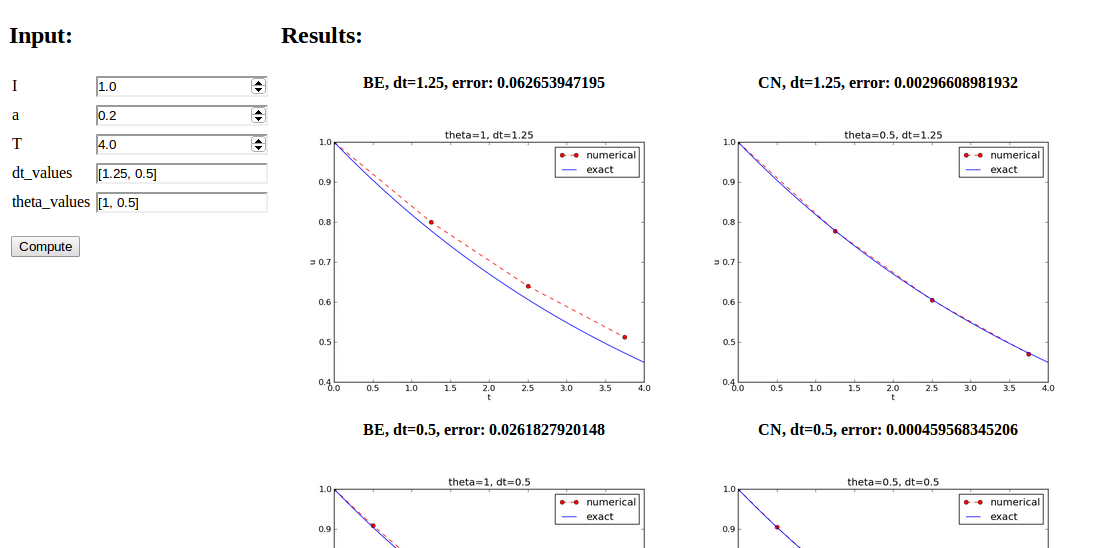
Automatically generated graphical web interface
Verification
Comparison with hand calculations
One of the simplest and most powerful methods for verifying numerical codes is to perform some steps of the algorithm by hand and compare the results with those produced by the code. In the present case, we may choose some test problem and run three steps by hand. Picking \(a(t)=t^2\)...
Test function
Caution: choice of parameter values
For the choice of values of parameters in verification tests one should stay away from integers, especially 0 and 1, as these can simplify formulas too much for test purposes. For example, with \(\theta =1\) the nominator in the formula for \(u^n\) will be the same for all \(a\) and \(\Delta t\) values. One should therefore choose more “arbitrary” values, say \(\theta =0.8\) and \(I=0.1\).
Comparison with an exact discrete solution
Sometimes it is possible to find a closed-form exact discrete solution that fulfills the discrete finite difference equations. The implementation can then be verified against the exact discrete solution. This is usually the best technique for verification.
Define
Manual computations with the \(\theta\)-rule results in
We have then established the exact discrete solution as
Caution
One should be conscious about the different meanings of the notation on the left- and right-hand side of (2): on the left, \(n\) in \(u^n\) is a superscript reflecting a counter of mesh points (\(t_n\)), while on the right, \(n\) is the power in the exponentiation \(A^n\).
Comparison of the exact discrete solution and the computed solution is done in the following function:
def verify_exact_discrete_solution():

    def exact_discrete_solution(n, I, a, theta, dt):
        A = (1 - (1-theta)*a*dt)/(1 + theta*dt*a)
        return I*A**n

    theta = 0.8; a = 2; I = 0.1; dt = 0.8
    Nt = int(8/dt)  # no of steps
    u, t = solver(I=I, a=a, T=Nt*dt, dt=dt, theta=theta)
    u_de = array([exact_discrete_solution(n, I, a, theta, dt)
                  for n in range(Nt+1)])
    difference = abs(u_de - u).max()  # max deviation
    tol = 1E-15  # tolerance for comparing floats
    success = difference <= tol
    return success
The complete program is found in the file decay_verf2.py (verf2 is a short name for “verification, version 2”).
Local functions
One can define a function inside another function, here called a local function (also known as closure) inside a parent function. A local function is invisible outside the parent function. A convenient property is that any local function has access to all variables defined in the parent function, also if we send the local function to some other function as argument (!). In the present example, it means that the local function exact_discrete_solution does not need its five arguments as the values can alternatively be accessed through the local variables defined in the parent function verify_exact_discrete_solution. We can send such an exact_discrete_solution without arguments to any other function and exact_discrete_solution will still have access to n, I, a, and so forth defined in its parent function.
Computing convergence rates
We expect that the error \(E\) in the numerical solution is reduced if the mesh size \(\Delta t\) is decreased. More specifically, many numerical methods obey a power-law relation between \(E\) and \(\Delta t\):
where \(C\) and \(r\) are (usually unknown) constants independent of \(\Delta t\). The formula (3) is viewed as an asymptotic model valid for sufficiently small \(\Delta t\). How small is normally hard to estimate without doing numerical estimations of \(r\).
The parameter \(r\) is known as the convergence rate. For example, if the convergence rate is 2, halving \(\Delta t\) reduces the error by a factor of 4. Diminishing \(\Delta t\) then has a greater impact on the error compared with methods that have \(r=1\). For a given value of \(r\), we refer to the method as of \(r\)-th order. First- and second-order methods are most common in scientific computing.
Estimating \(r\)
There are two alternative ways of estimating \(C\) and \(r\) based on a set of \(m\) simulations with corresponding pairs \((\Delta t_i, E_i)\), \(i=0,\ldots,m-1\), and \(\Delta t_{i} < \Delta t_{i-1}\) (i.e., decreasing cell size).
- Take the logarithm of (3), \(\ln E = r\ln \Delta t + \ln C\), and fit a straight line to the data points \((\Delta t_i, E_i)\), \(i=0,\ldots,m-1\).
- Consider two consecutive experiments, \((\Delta t_i, E_i)\) and \((\Delta t_{i-1}, E_{i-1})\). Dividing the equation \(E_{i-1}=C\Delta t_{i-1}^r\) by \(E_{i}=C\Delta t_{i}^r\) and solving for \(r\) yields
for \(i=1,\ldots,m-1\).
The disadvantage of method 1 is that (3) might not be valid for the coarsest meshes (largest \(\Delta t\) values). Fitting a line to all the data points is then misleading. Method 2 computes convergence rates for pairs of experiments and allows us to see if the sequence \(r_i\) converges to some value as \(i\rightarrow m-2\). The final \(r_{m-2}\) can then be taken as the convergence rate. If the coarsest meshes have a differing rate, the corresponding time steps are probably too large for (3) to be valid. That is, those time steps lie outside the asymptotic range of \(\Delta t\) values where the error behaves like (3).
Implementation (2)
It is straightforward to extend the main function in the program decay_argparse.py with statements for computing \(r_0, r_1, \ldots, r_{m-2}\) from (3):
from math import log

def main():
    I, a, T, makeplot, dt_values = read_command_line()
    r = {}  # estimated convergence rates
    for theta in 0, 0.5, 1:
        E_values = []
        for dt in dt_values:
            E = explore(I, a, T, dt, theta, makeplot=False)
            E_values.append(E)

        # Compute convergence rates
        m = len(dt_values)
        r[theta] = [log(E_values[i-1]/E_values[i])/
                    log(dt_values[i-1]/dt_values[i])
                    for i in range(1, m, 1)]

    for theta in r:
        print '\nPairwise convergence rates for theta=%g:' % theta
        print ' '.join(['%.2f' % r_ for r_ in r[theta]])
    return r
The program containing this main function is called decay_convrate.py.
The r object is a dictionary of lists. The keys in this dictionary are the \(\theta\) values. For example, r[1] holds the list of the \(r_i\) values corresponding to \(\theta=1\). In the loop for theta in r, the loop variable theta takes on the values of the keys in the dictionary r (in an undetermined ordering). We could simply do a print r[theta] inside the loop, but this would typically yield output of the convergence rates with 16 decimals:
[1.331919482274763, 1.1488178494691532, ...]
Instead, we format each number with 2 decimals, using a list comprehension to turn the list of numbers, r[theta], into a list of formatted strings. Then we join these strings with a space in between to get a sequence of rates on one line in the terminal window. More generally, d.join(list) joins the strings in the list list to one string, with d as delimiter between list[0], list[1], etc.
Here is an example on the outcome of the convergence rate computations:
Terminal> python decay_convrate.py --dt 0.5 0.25 0.1 0.05 0.025 0.01
...
Pairwise convergence rates for theta=0:
1.33 1.15 1.07 1.03 1.02

Pairwise convergence rates for theta=0.5:
2.14 2.07 2.03 2.01 2.01

Pairwise convergence rates for theta=1:
0.98 0.99 0.99 1.00 1.00
The Forward and Backward Euler methods seem to have an \(r\) value which stabilizes at 1, while the Crank-Nicolson seems to be a second-order method with \(r=2\).
Very often, we have some theory that predicts what \(r\) is for a numerical method. Various theoretical error measures for the \(\theta\)-rule point to \(r=2\) for \(\theta =0.5\) and \(r=1\) otherwise. The computed estimates of \(r\) are in very good agreement with these theoretical values.
Why convergence rates are important
The strong practical application of computing convergence rates is for verification: wrong convergence rates point to errors in the code, and correct convergence rates brings evidence that the implementation is correct. Experience shows that bugs in the code easily destroy the expected convergence rate.
Debugging via convergence rates
Let us experiment with bugs and see the implication on the convergence rate. We may, for instance, forget to multiply by a in the denominator in the updating formula for u[n+1]:
u[n+1] = (1 - (1-theta)*a*dt)/(1 + theta*dt)*u[n]
Running the same decay_convrate.py command as above gives the expected convergence rates (!). Why? The reason is that we just specified the \(\Delta t\) values are relied on default values for other parameters. The default value of \(a\) is 1. Forgetting the factor a has then no effect. This example shows how important it is to avoid parameters that are 1 or 0 when verifying implementations. Running the code decay_v0.py with \(a=2.1\) and \(I=0.1\) yields
Terminal> python decay_convrate.py --a 2.1 --I 0.1  \
          --dt 0.5 0.25 0.1 0.05 0.025 0.01
...
Pairwise convergence rates for theta=0:
1.49 1.18 1.07 1.04 1.02

Pairwise convergence rates for theta=0.5:
-1.42 -0.22 -0.07 -0.03 -0.01

Pairwise convergence rates for theta=1:
0.21 0.12 0.06 0.03 0.01
This time we see that the expected convergence rates for the Crank-Nicolson and Backward Euler methods are not obtained, while \(r=1\) for the Forward Euler method. The reason for correct rate in the latter case is that \(\theta=0\) and the wrong theta*dt term in the denominator vanishes anyway.
The error
u[n+1] = ((1-theta)*a*dt)/(1 + theta*dt*a)*u[n]
manifests itself through wrong rates \(r\approx 0\) for all three methods. About the same results arise from an erroneous initial condition, u[0] = 1, or wrong loop limits, range(1,Nt). It seems that in this simple problem, most bugs we can think of are detected by the convergence rate test, provided the values of the input data do not hide the bug.
A verify_convergence_rate function could compute the dictionary of list via main and check if the final rate estimates (\(r_{m-2}\)) are sufficiently close to the expected ones. A tolerance of 0.1 seems appropriate, given the uncertainty in estimating \(r\):
def verify_convergence_rate():
    r = main()
    tol = 0.1
    expected_rates = {0: 1, 1: 1, 0.5: 2}
    for theta in r:
        r_final = r[theta][-1]
        diff = abs(expected_rates[theta] - r_final)
        if diff > tol:
            return False
    return True  # all tests passed
We remark that r[theta] is a list and the last element in any list can be extracted by the index -1.
![]()
Table Of Contents
Previous topic
Scientific software engineering with a simple ODE model as example
