Ch.5: Array computing and curve plotting
Aug 21, 2016
Goal: learn to visualize functions

We need to learn about a new object: array
- Curves \( y=f(x) \) are visualized by drawing straight lines between points along the curve
- Meed to store the coordinates of the points along the curve in lists or arrays
xandy - Arrays \( \approx \) lists, but computationally much more efficient
- To compute the
ycoordinates (in an array) we need to learn about array computations or vectorization - Array computations are useful for much more than plotting curves!
The minimal need-to-know about vectors
- Vectors are known from high school mathematics, e.g.,
point \( (x,y) \) in the plane, point \( (x,y,z) \) in space - In general, a vector \( v \) is an \( n \)-tuple of numbers:
\( v=(v_0,\ldots,v_{n-1}) \) - Vectors can be represented by lists: \( v_i \) is stored as
v[i],
but we shall use arrays instead
Vectors and arrays are key concepts in this chapter. It takes separate math courses to understand what vectors and arrays really are, but in this course we only need a small subset of the complete story. A learning strategy may be to just start using vectors/arrays in programs and later, if necessary, go back to the more mathematical details in the first part of Ch. 5.
The minimal need-to-know about arrays
Arrays are a generalization of vectors where we can have multiple indices: \( A_{i,j} \), \( A_{i,j,k} \)
Example: table of numbers, one index for the row, one for the column
$$
\left\lbrack\begin{array}{cccc}
0 & 12 & -1 & 5\\
-1 & -1 & -1 & 0\\
11 & 5 & 5 & -2
\end{array}\right\rbrack
\hspace{1cm}
A =
\left\lbrack\begin{array}{ccc}
A_{0,0} & \cdots & A_{0,n-1}\\
\vdots & \ddots & \vdots\\
A_{m-1,0} & \cdots & A_{m-1,n-1}
\end{array}\right\rbrack
$$
- The no of indices in an array is the rank or number of dimensions
- Vector = one-dimensional array, or rank 1 array
- In Python code, we use Numerical Python arrays instead of nested lists to represent mathematical arrays (because this is computationally more efficient)
Storing (x,y) points on a curve in lists
>>> def f(x):
...     return x**3
...
>>> n = 5                 # no of points
>>> dx = 1.0/(n-1)        # x spacing in [0,1]
>>> xlist = [i*dx for i in range(n)]
>>> ylist = [f(x) for x in xlist]

>>> pairs = [[x, y] for x, y in zip(xlist, ylist)]
>>> import numpy as np        # module for arrays
>>> x = np.array(xlist)      # turn list xlist into array
>>> y = np.array(ylist)
Make arrays directly (instead of lists)
>>> n = 5                     # number of points
>>> x = np.linspace(0, 1, n) # n points in [0, 1]
>>> y = np.zeros(n)          # n zeros (float data type)
>>> for i in xrange(n):
...     y[i] = f(x[i])
...
Note:
-
xrangeis likerangebut faster (esp. for largen-xrangedoes not explicitly build a list of integers,xrangejust lets you loop over the values) - Entire arrays must be made by
numpy(np) functions
Arrays are not as flexible as list, but computational much more efficient
- List elements can be any Python objects
- Array elements can only be of one object type
- Arrays are very efficient to store in memory and compute with
if the element type isfloat,int, orcomplex - Rule: use arrays for sequences of numbers!
We can work with entire arrays at once - instead of one element at a time
Compute the sine of an array:
from math import sin

for i in xrange(len(x)):
    y[i] = sin(x[i])
However, if x is array, y can be computed by
y = np.sin(x) # x: array, y: array
The loop is now inside np.sin and implemented in very efficient C code.
Operating on entire arrays at once is called vectorization
- shorter, more readable code, closer to the mathematics
- much faster code
%timeit in IPython to measure the speed-up for \( y=\sin x e^{-x} \):
In [1]: n = 100000

In [2]: import numpy as np

In [3]: x = np.linspace(0, 2*np.pi, n+1)

In [4]: y = np.zeros(len(x))

In [5]: %timeit for i in xrange(len(x)): \
        y[i] = np.sin(x[i])*np.exp(-x[i])
1 loops, best of 3: 247 ms per loop

In [6]: %timeit y = np.sin(x)*np.exp(-x)
100 loops, best of 3: 4.77 ms per loop

In [7]: 247/4.77
Out[7]: 51.781970649895186  # vectorization: 50x speed-up!
A function f(x) written for a number x usually works for array x too
from numpy import sin, exp, linspace

def f(x):
    return x**3 + sin(x)*exp(-3*x)

x = 1.2                     # float object
y = f(x)                    # y is float

x = linspace(0, 3, 10001)   # 10000 intervals in [0,3]
y = f(x)                    # y is array
math is for numbers and numpy for arrays.
>>> import math, numpy
>>> x = numpy.linspace(0, 1, 11)
>>> math.sin(x[3])
0.2955202066613396
>>> math.sin(x)
...
TypeError: only length-1 arrays can be converted to Python scalars
>>> numpy.sin(x)
array([ 0.     ,  0.09983,  0.19866,  0.29552,  0.38941,
        0.47942,  0.56464,  0.64421,  0.71735,  0.78332,
        0.84147])
Array arithmetics is broken down to a series of unary/binary array operations
- Consider
y = f(x), wherefreturnsx**3 + sin(x)*exp(-3*x) -
f(x)leads to the following set of vectorized sub-computations: -
r1 = x**3
for i in range(len(x)): r1[i] = x[i]**3
(but with loop in C) -
r2 = sin(x)(computed elementwise in C) -
r3 = -3*x -
r4 = exp(r3) -
r5 = r3*r4 -
r6 = r1 + r5 -
y = r6 - Note: this is the same set of operations as you would do with a calculator
when
xis a number
Very important application: vectorized code for computing points along a curve
$$ f(x) = x^2e^{-\frac{1}{2}x}\sin(x-\frac{1}{3}\pi),\quad x\in [0, 4\pi]$$
from numpy import *

n = 100
x = linspace(0, 4*pi, n+1)
y = 2.5 + x**2*exp(-0.5*x)*sin(x-pi/3)
New term: vectorization
- Scalar: a number
- Vector or array: sequence of numbers (vector in mathematics)
- We speak about scalar computations (one number at a time) versus vectorized computations (operations on entire arrays, no Python loops)
- Vectorized functions can operate on arrays (vectors)
- Vectorization is the process of turning a non-vectorized algorithm with (Python) loops into a vectorized version without (Python) loops
- Mathematical functions in Python without
iftests automatically work for both scalar and vector (array) arguments (i.e., no vectorization is needed by the programmer)
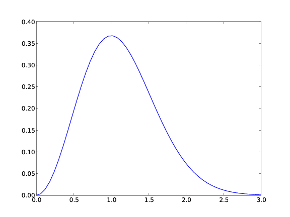
Plotting the curve of a function: the very basics
from scitools.std import *  # import numpy and plotting

# Make points along the curve
t = linspace(0, 3, 51)      # 50 intervals in [0, 3]
y = t**2*exp(-t**2)         # vectorized expression

plot(t, y)           # make plot on the screen
savefig('fig.pdf')   # make PDF image for reports
savefig('fig.png')   # make PNG image for web pages
A plot should have labels on axis and a title
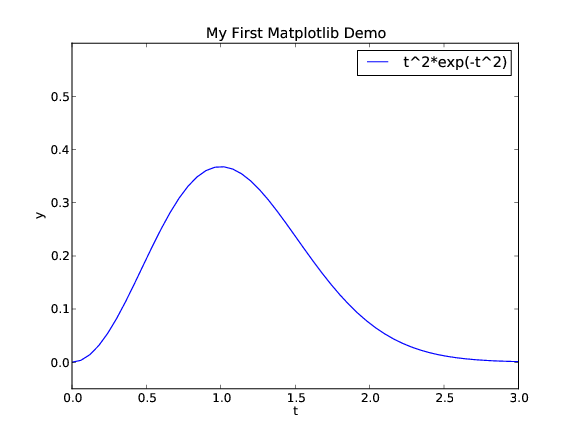
The code that makes the last plot
from scitools.std import *  # import numpy and plotting

def f(t):
    return t**2*exp(-t**2)

t = linspace(0, 3, 51)    # t coordinates
y = f(t)                  # corresponding y values

plot(t, y)

xlabel('t')               # label on the x axis
ylabel('y')               # label on the y axix
legend('t^2*exp(-t^2)')   # mark the curve
axis([0, 3, -0.05, 0.6])  # [tmin, tmax, ymin, ymax]
title('My First Easyviz Demo')
SciTools vs. NumPy and Matplotlib
- SciTools is a Python package with lots of useful tools for mathematical computations, developed here in Oslo (Langtangen, Ring, Wilbers, Bredesen, ...)
- Easyviz is a subpackage of SciTools (
scitools.easyviz) doing plotting with Matlab-like syntax - Easyviz can use many plotting engine to produce a plot: Matplotlib, Gnuplot, Grace, Matlab, VTK, OpenDx, ... but the syntax remains the same
- Matplotlib is the standard plotting package in the Python community - Easyviz can use the same syntax as Matplotlib
from scitools.std import *

# is basically equivalent to

from numpy import *
from matplotlib.pyplot import *
Note: SciTools (by default) adds markers to the lines, Matplotlib does not
Easyviz (imported from scitools.std) allows a more compact "Pythonic" syntax for plotting curves
Use keyword arguments instead of separate function calls:
plot(t, y,
     xlabel='t',
     ylabel='y',
     legend='t^2*exp(-t^2)',
     axis=[0, 3, -0.05, 0.6],
     title='My First Easyviz Demo',
     savefig='tmp1.png',
     show=True)   # display on the screen (default)
(This cannot be done with Matplotlib.)
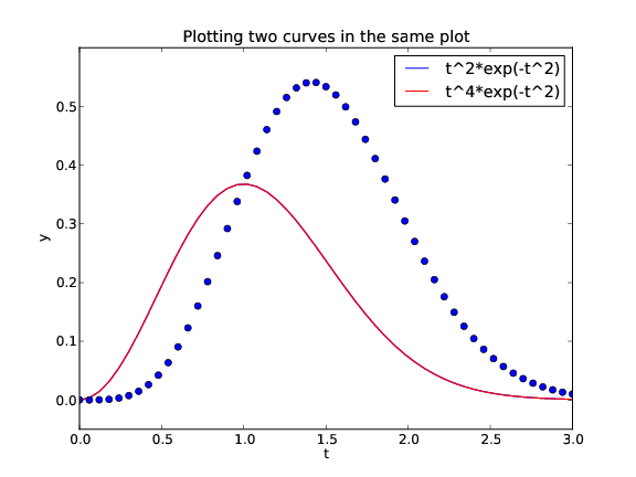
Plotting several curves in one plot
from scitools.std import *   # curve plotting + array computing

def f1(t):
    return t**2*exp(-t**2)

def f2(t):
    return t**2*f1(t)

t = linspace(0, 3, 51)
y1 = f1(t)
y2 = f2(t)

plot(t, y1)
hold('on')   # continue plotting in the same plot
plot(t, y2)

xlabel('t')
ylabel('y')
legend('t^2*exp(-t^2)', 't^4*exp(-t^2)')
title('Plotting two curves in the same plot')
savefig('tmp2.png')
Alternative, more compact plot command
plot(t, y1, t, y2,
     xlabel='t', ylabel='y',
     legend=('t^2*exp(-t^2)', 't^4*exp(-t^2)'),
     title='Plotting two curves in the same plot',
     savefig='tmp2.pdf')

# equivalent to
plot(t, y1)
hold('on')
plot(t, y2)

xlabel('t')
ylabel('y')
legend('t^2*exp(-t^2)', 't^4*exp(-t^2)')
title('Plotting two curves in the same plot')
savefig('tmp2.pdf')
The resulting plot with two curves
Controlling line styles
When plotting multiple curves in the same plot, the different lines (normally) look different. We can control the line type and color, if desired:
plot(t, y1, 'r-')   # red (r) line (-)
hold('on')
plot(t, y2, 'bo')   # blue (b) circles (o)

# or
plot(t, y1, 'r-', t, y2, 'bo')
Documentation of colors and line styles: see the book, Ch. 5, or
Unix> pydoc scitools.easyviz
Quick plotting with minimal typing
t = linspace(0, 3, 51)
plot(t, t**2*exp(-t**2), t, t**4*exp(-t**2))
Plot function given on the command line
Terminal> python plotf.py expression xmin xmax
Terminal> python plotf.py "exp(-0.2*x)*sin(2*pi*x)" 0 4*pi
Should plot \( e^{-0.2x}\sin (2\pi x) \), \( x\in [0,4\pi] \).
plotf.py should work for "any" mathematical expression.
Solution
from scitools.std import *
# or alternatively
from numpy import *
from matplotlib.pyplot import *

formula = sys.argv[1]
xmin = eval(sys.argv[2])
xmax = eval(sys.argv[3])

x = linspace(xmin, xmax, 101)
y = eval(formula)
plot(x, y, title=formula)
Let's make a movie/animation
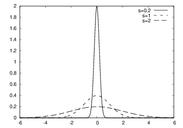
The Gaussian/bell function
|
|
|
Movies are made from a (large) set of individual plots
- Goal: make a movie showing how \( f(x) \) varies in shape as \( s \) decreases
- Idea: put many plots (for different \( s \) values) together
(exactly as a cartoon movie) - How to program: loop over \( s \) values, call
plotfor each \( s \) and make hardcopy, combine all hardcopies to a movie - Very important: fix the \( y \) axis! Otherwise, the \( y \) axis always adapts to the peak of the function and the visual impression gets completely wrong
The complete code for making the animation
from scitools.std import *
import time

def f(x, m, s):
    return (1.0/(sqrt(2*pi)*s))*exp(-0.5*((x-m)/s)**2)

m = 0;  s_start = 2;  s_stop = 0.2
s_values = linspace(s_start, s_stop, 30)

x = linspace(m -3*s_start, m + 3*s_start, 1000)
# f is max for x=m (smaller s gives larger max value)
max_f = f(m, m, s_stop)

# Show the movie on the screen
# and make hardcopies of frames simultaneously
import time
frame_counter = 0

for s in s_values:
    y = f(x, m, s)
    plot(x, y, axis=[x[0], x[-1], -0.1, max_f],
         xlabel='x', ylabel='f', legend='s=%4.2f' % s,
         savefig='tmp_%04d.png' % frame_counter)
    frame_counter += 1
    #time.sleep(0.2)  # pause to control movie speed
How to combine plot files to a movie (video file)
We now have a lot of files:
tmp_0000.png tmp_0001.png tmp_0002.png ...
We use some program to combine these files to a video file:
-
convertfor animted GIF format (if just a few plot files) -
ffmpeg(oravconv) for MP4, WebM, Ogg, and Flash formats
Make and play animated GIF file
Tool: convert from the ImageMagick software suite.
Unix command:
Terminal> convert -delay 50 tmp_*.png movie.gif
Delay: 50/100 s, i.e., 0.5 s between each frame.
Play animated GIF file with animate from ImageMagick:
Terminal> animate movie.gif
or insert this HTML code in some file tmp.html loaded into a browser:
<img src="movie.gif">
Making MP4, Ogg, WebM, or Flash videos
Tool: ffmpeg or avconv
Terminal> ffmpeg -r 5 -i tmp_%04d.png -vcodec flv movie.flv
where
-
-r 5specifies 5 frames per second -
-i tmp_%04d.pngspecifies filenames
(tmp_0000.png,tmp_0001.png, ...)
Different formats apply different codecs (-vcodec) and
video filenamet extensions:
| Format | Codec and filename |
|---|---|
| Flash | -vcodec flv movie.flv |
| MP4 | -vcodec libx264 movie.mp4 |
| Webm | -vcodec libvpx movie.webm |
| Ogg | -vcodec libtheora movie.ogg |
How to play movie files in general (with vlc)
Terminal> vlc movie.flv
Terminal> vlc movie.ogg
Terminal> vlc movie.webm
Terminal> vlc movie.mp4
Other players (on Linux) are mplayer, totem, ...
HTML PNG file player
Terminal> scitools movie output_file=mymovie.html fps=4 tmp_*.png
makes a player of tmp_*.png files in a file mymovie.html
(load into a web browser)
It is possible to plot curves in pure text (!)
- Plots are stored in image files of type PDF and PNG
- Sometimes you want a plot to be included in your program,
e.g., to prove that the curve looks right in a compulsory exercise where only the program (and not a nicely typeset report) is submitted -
scitools.aplottercan then be used for drawing primitive curves in pure text (ASCII) format
>>> from scitools.aplotter import plot
>>> from numpy import linspace, exp, cos, pi
>>> x = linspace(-2, 2, 81)
>>> y = exp(-0.5*x**2)*cos(pi*x)
>>> plot(x, y)
Try these statements out!
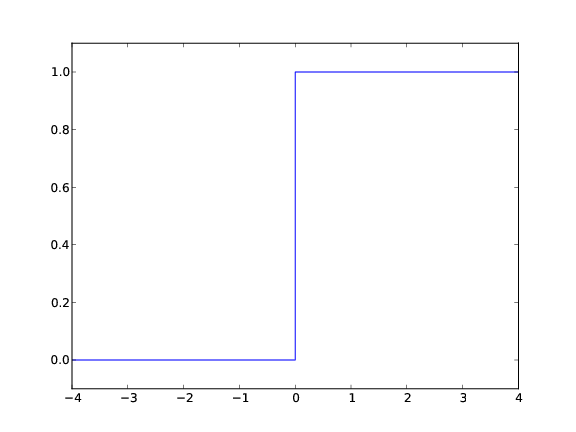
Let's try to plot a discontinuous function
The Heaviside function is frequently used in science and engineering:
$$ H(x) = \left\lbrace\begin{array}{ll}
0, & x < 0\\
1, & x\geq 0
\end{array}\right.
$$
Python implementation:
def H(x):
    return (0 if x < 0 else 1)
Plotting the Heaviside function: first try
x = linspace(-10, 10, 5)  # few points (simple curve)
y = H(x)
plot(x, y)
First problem: ValueError error in H(x) from if x < 0
Let us debug in an interactive shell:
>>> x = linspace(-10,10,5)
>>> x
array([-10.,  -5.,   0.,   5.,  10.])
>>> b = x < 0
>>> b
array([ True,  True, False, False, False], dtype=bool)
>>> bool(b)  # evaluate b in a boolean context
...
ValueError: The truth value of an array with more than
one element is ambiguous. Use a.any() or a.all()
if x < 0 does not work if x is array
x values.
def H_loop(x):
    r = zeros(len(x))  # or r = x.copy()
    for i in xrange(len(x)):
        r[i] = H(x[i])
    return r

n = 5
x = linspace(-5, 5, n+1)
y = H_loop(x)
Downside: much to write, slow code if n is large
if x < 0 does not work if x is array
vectorize.
from numpy import vectorize

# Automatic vectorization of function H
Hv = vectorize(H)
# Hv(x) works with array x
Downside: The resulting function is as slow as Remedy 1
if x < 0 does not work if x is array
if test differently.
def Hv(x):
    return where(x < 0, 0.0, 1.0)
def f(x):
    if condition:
        x = <expression1>
    else:
        x = <expression2>
    return x

def f_vectorized(x):
def f_vectorized(x):
    x1 = <expression1>
    x2 = <expression2>
    r = np.where(condition, x1, x2)
    return r
Back to plotting the Heaviside function
With a vectorized Hv(x) function we can plot in the standard way
x = linspace(-10, 10, 5)   # linspace(-10, 10, 50)
y = Hv(x)
plot(x, y, axis=[x[0], x[-1], -0.1, 1.1])
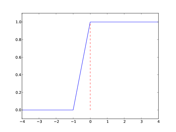
How to make the function look discontinuous in the plot?
- Newbie: use a lot of \( x \) points; the curve gets steeper
- Pro: plot just two horizontal line segments
one from \( x=-10 \) to \( x=0 \), \( y=0 \); and one from \( x=0 \) to \( x=10 \), \( y=1 \)
plot([-10, 0, 0, 10], [0, 0, 1, 1],
     axis=[x[0], x[-1], -0.1, 1.1])
Draws straight lines between \( (-10,0) \), \( (0,0) \), \( (0,1) \), \( (10, 1) \)
The final plot of the discontinuous Heaviside function
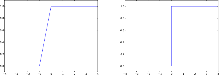
Removing the vertical jump from the plot
Some will argue and say that at high school they would draw \( H(x) \) as two horizontal lines without the vertical line at \( x=0 \), illustrating the jump. How can we plot such a curve?
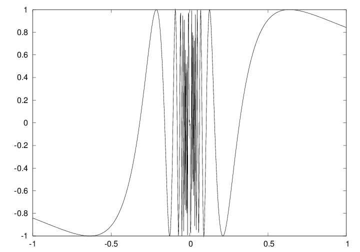
Some functions are challenging to visualize
def f(x):
    return sin(1.0/x)

x1 = linspace(-1, 1, 10)    # use 10 points
x2 = linspace(-1, 1, 1000)  # use 1000 points
plot(x1, f(x1), label='%d points' % len(x))
plot(x2, f(x2), label='%d points' % len(x))
Plot based on 10 points
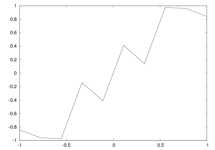
Plot based on 1000 points
Assignment of an array does not copy the elements!
a = x
a[-1] = 1000
Is x[-1] also changed to 1000?
Yes, because a refers to the same array as x.
Avoid changing x by letting a be a copy of x:
a = x.copy()
The same yields slices:
a = x[r:]      # a refers to a part of the x array
a[-1] = 1000   # changes x[-1]!
a = x[r:].copy()
a[-1] = 1000   # does not change x[-1]
In-place array arithmetics
The two following statements are mathematically equivalent:
a = a + b    # a and b are arrays
a += b
However,
-
a = a + bis computed as (extra array needed) -
r1 = a + b -
a = r1 -
a += bis computed asa[i] += b[i]foriin all indices (i.e., not extra array) -
a += bis an in-place addition, because we change each element ina, rather than letting the namearefer to a new array, the result ofa+b
In-place array arithmetics can save memory demands
Consider
a = (3*x**4 + 2*x + 4)/(x + 1)
Here are the actual computations in the computer:
r1 = x**4;  r2 = 3*r1;  r3 = 2*x;  r4 = r1 + r3
r5 = r4 + 4;  r6 = x + 1; r7 = r5/r6; a = r7
With in-place arithmetics we can save four extra arrays, though at the cost of much less readable code:
a = x.copy()
a **= 4
a *= 3
a += 2*x
a += 4
a /= x + 1
In-place arithmetics only saves memory, no significant speed-up
Let's use IPython to measure the computational time:
In [1]: def expression(x):
   ...:     return (3*x**4 + 2*x + 4)/(x + 1)
   ...:

In [2]: def expression_inplace(x):
   ...:     a = x.copy()
   ...:     a **= 4
   ...:     a *= 3
   ...:     a += 2*x
   ...:     a += 4
   ...:     a /= x + 1
   ...:     return a
   ...:

In [3]: import numpy as np

In [4]: x = np.linspace(0, 1, 10000000)

In [5]: %timeit  expression(x)
1 loops, best of 3: 771 ms per loop

In [6]: %timeit  expression_inplace(x)
1 loops, best of 3: 728 ms per loop
Only 5% speed-up, so use +=, -=, etc. when arrays are large and
you need to save memory
Useful array operations
Make a new array with same size as another array:
from numpy import *

# x is numpy array
a = x.copy()

# or
a = zeros(x.shape, x.dtype)

# or
a = zeros_like(x)  # zeros and same size as x
Make sure a list or array is an array:
a = asarray(a)
b = asarray(somearray, dtype=float)  # specify data type
Test if an object is an array:
>>> type(a)
<type 'numpy.ndarray'>
>>> isinstance(a, ndarray)
True
Example: vectorizing a constant function
def f(x):
    return 2
Vectorized version must return array of 2's:
def fv(x):
    return zeros(x.shape, x.dtype) + 2
New version valid both for scalar and array x:
def f(x):
    if isinstance(x, (float, int)):
        return 2
    elif isinstance(x, ndarray):
        return zeros(x.shape, x.dtype) + 2
    else:
        raise TypeError(
           'x must be int/float/ndarray, not %s' % type(x))
Generalized array indexing
Recall slicing: a[f:t:i], where the slice f:t:i implies a set of indices
(from, to, increment).
Any integer list or array can be used to indicate a set of indices:
>>> a = linspace(1, 8, 8)
>>> a
array([ 1.,  2.,  3.,  4.,  5.,  6.,  7.,  8.])
>>> a[[1,6,7]] = 10
>>> a
array([  1.,  10.,   3.,   4.,   5.,   6.,  10.,  10.])
>>> a[range(2,8,3)] = -2   # same as a[2:8:3] = -2
>>> a
array([  1.,  10.,  -2.,   4.,   5.,  -2.,  10.,  10.])
Generalized array indexing with boolean expressions
>>> a < 0
[False, False, True, False, False, True, False, False]

>>> a[a < 0]           # pick out all negative elements
array([-2., -2.])

>>> a[a < 0] = a.max() # if a[i]<10, set a[i]=10
>>> a
array([  1.,  10.,  10.,   4.,   5.,  10.,  10.,  10.])
Two-dimensional arrays; math intro
When we have a table of numbers,
$$
\left\lbrack\begin{array}{cccc}
0 & 12 & -1 & 5\\
-1 & -1 & -1 & 0\\
11 & 5 & 5 & -2
\end{array}\right\rbrack
$$
(called matrix by mathematicians) it is natural to use a two-dimensional array \( A_{i,j} \) with one index for the rows and one for the columns:
$$
A =
\left\lbrack\begin{array}{ccc}
A_{0,0} & \cdots & A_{0,n-1}\\
\vdots & \ddots & \vdots\\
A_{m-1,0} & \cdots & A_{m-1,n-1}
\end{array}\right\rbrack
$$
Two-dimensional arrays; Python code
Making and filling a two-dimensional NumPy array goes like this:
A = zeros((3,4))   # 3x4 table of numbers
A[0,0] = -1
A[1,0] =  1
A[2,0] = 10
A[0,1] = -5
...
A[2,3] = -100

# can also write (as for nested lists)
A[2][3] = -100
From nested list to two-dimensional array
Let us make a table of numbers in a nested list:
>>> Cdegrees = [-30 + i*10 for i in range(3)]
>>> Fdegrees = [9./5*C + 32 for C in Cdegrees]
>>> table = [[C, F] for C, F in zip(Cdegrees, Fdegrees)]
>>> print table
[[-30, -22.0], [-20, -4.0], [-10, 14.0]]
Turn into NumPy array:
>>> table2 = array(table)
>>> print table2
[[-30. -22.]
 [-20.  -4.]
 [-10.  14.]]
How to loop over two-dimensional arrays
>>> table2.shape   # see the number of elements in each dir.
(3, 2)             # 3 rows, 2 columns
A for loop over all array elements:
>>> for i in range(table2.shape[0]):
...     for j in range(table2.shape[1]):
...         print 'table2[%d,%d] = %g' % (i, j, table2[i,j])
...
table2[0,0] = -30
table2[0,1] = -22
...
table2[2,1] = 14
Alternative single loop over all elements:
>>> for index_tuple, value in np.ndenumerate(table2):
...     print 'index %s has value %g' % \
...           (index_tuple, table2[index_tuple])
...
index (0,0) has value -30
index (0,1) has value -22
...
index (2,1) has value 14
>>> type(index_tuple)
<type 'tuple'>
How to take slices of two-dimensional arrays
Rule: can use slices start:stop:inc for each index
table2[0:table2.shape[0], 1]  # 2nd column (index 1)
array([-22.,  -4.,  14.])

>>> table2[0:, 1]             # same
array([-22.,  -4.,  14.])

>>> table2[:, 1]              # same
array([-22.,  -4.,  14.])

>>> t = linspace(1, 30, 30).reshape(5, 6)
>>> t[1:-1:2, 2:]
array([[  9.,  10.,  11.,  12.],
       [ 21.,  22.,  23.,  24.]])
>>> t
array([[  1.,   2.,   3.,   4.,   5.,   6.],
       [  7.,   8.,   9.,  10.,  11.,  12.],
       [ 13.,  14.,  15.,  16.,  17.,  18.],
       [ 19.,  20.,  21.,  22.,  23.,  24.],
       [ 25.,  26.,  27.,  28.,  29.,  30.]])
Time for a question
Given
>>> t
array([[  1.,   2.,   3.,   4.,   5.,   6.],
       [  7.,   8.,   9.,  10.,  11.,  12.],
       [ 13.,  14.,  15.,  16.,  17.,  18.],
       [ 19.,  20.,  21.,  22.,  23.,  24.],
       [ 25.,  26.,  27.,  28.,  29.,  30.]])
What will t[1:-1:2, 2:] be?
Slice 1:-1:2 for first index results in
[  7.,   8.,   9.,  10.,  11.,  12.]
[ 19.,  20.,  21.,  22.,  23.,  24.]
Slice 2: for the second index then gives
[  9.,  10.,  11.,  12.]
[ 21.,  22.,  23.,  24.]
Summary of vectors and arrays
- Vector/array computing: apply a mathematical expression to every element in the vector/array (no loops in Python)
- Ex:
sin(x**4)*exp(-x**2),xcan be array or scalar
for array thei'th element becomessin(x[i]**4)*exp(-x[i]**2) - Vectorization: make scalar mathematical computation valid for vectors/arrays
- Pure mathematical expressions require no extra vectorization
- Mathematical formulas involving
iftests require manual work for vectorization:
scalar_result = expression1 if condition else expression2
vector_result = where(condition, expression1, expression2)
Summary of plotting \( y=f(x) \) curves
Curve plotting (unified syntax for Matplotlib and SciTools):
from matplotlib.pyplot import *
#from scitools.std import *


plot(x, y)         # simplest command

plot(t1, y1, 'r',  # curve 1, red line
     t2, y2, 'b',  # curve 2, blue line
     t3, y3, 'o')  # curve 3, circles at data points
axis([t1[0], t1[-1], -1.1, 1.1])
legend(['model 1', 'model 2', 'measurements'])
xlabel('time');  ylabel('force')
savefig('myframe_%04d.png' % plot_counter)
Note: straight lines are drawn between each data point
Alternativ plotting of \( y=f(x) \) curves
Single SciTools plot command with keyword arguments:
from scitools.std import *

plot(t1, y1, 'r',  # curve 1, red line
     t2, y2, 'b',  # curve 2, blue line
     t3, y3, 'o',  # curve 3, circles at data points
     axis=[t1[0], t1[-1], -1.1, 1.1],
     legend=('model 1', 'model 2', 'measurements'),
     xlabel='time', ylabel='force',
     savefig='myframe_%04d.png' % plot_counter)
Summary of making animations
- Make a hardcopy of each plot frame (PNG or PDF format)
- Use
avconvorffmpegto make movie
Terminal> avconv -r 5 -i tmp_%04d.png -vcodec flv movie.flv
Array functionality
| Construction | Meaning |
|---|---|
array(ld) | copy list data ld to a numpy array |
asarray(d) | make array of data d (no data copy if already array) |
zeros(n) | make a float vector/array of length n, with zeros |
zeros(n, int) | make an int vector/array of length n with zeros |
zeros((m,n)) | make a two-dimensional float array with shape (m,`n`) |
zeros_like(x) | make array of same shape and element type as x |
linspace(a,b,m) | uniform sequence of m numbers in \( [a,b] \) |
a.shape | tuple containing a's shape |
a.size | total no of elements in a |
len(a) | length of a one-dim. array a (same as a.shape[0]) |
a.dtype | the type of elements in a |
a.reshape(3,2) | return a reshaped as \( 3\times 2 \) array |
a[i] | vector indexing |
a[i,j] | two-dim. array indexing |
a[1:k] | slice: reference data with indices 1,\ldots,`k-1` |
a[1:8:3] | slice: reference data with indices 1, 4,\ldots,`7` |
b = a.copy() | copy an array |
sin(a), exp(a), ... | numpy functions applicable to arrays |
c = concatenate((a, b)) | c contains a with b appended |
c = where(cond, a1, a2) | c[i] = a1[i] if cond[i], else c[i] = a2[i] |
isinstance(a, ndarray) | is True if a is an array |
Summarizing example: animating a function (part 1)
Goal: visualize the temperature in the ground as a function of depth (\( z \)) and time (\( t \)), displayed as a movie in time:
$$ T(z,t) = T_0 + Ae^{-az}\cos (\omega t - az),\quad a =\sqrt{\omega\over 2k} $$
First we make a general animation function for an \( f(x,t) \):
from scitools.std import plot  # convenient for animations

def animate(tmax, dt, x, function, ymin, ymax, t0=0,
            xlabel='x', ylabel='y', filename='tmp_'):
    t = t0
    counter = 0
    while t <= tmax:
        y = function(x, t)
        plot(x, y,
             axis=[x[0], x[-1], ymin, ymax],
             title='time=%g' % t,
             xlabel=xlabel, ylabel=ylabel,
             savefig=filename + '%04d.png' % counter)
        t += dt
        counter += 1
Then we call this function with our special \( T(z,t) \) function
Summarizing example: animating a function (part 2)
# remove old plot files:
import glob, os
for filename in glob.glob('tmp_*.png'): os.remove(filename)

def T(z, t):
    # T0, A, k, and omega are global variables
    a = sqrt(omega/(2*k))
    return T0 + A*exp(-a*z)*cos(omega*t - a*z)

k = 1E-6     # heat conduction coefficient (in m*m/s)
P = 24*60*60.# oscillation period of 24 h (in seconds)
omega = 2*pi/P
dt = P/24    # time lag: 1 h
tmax = 3*P   # 3 day/night simulation
T0 = 10      # mean surface temperature in Celsius
A = 10       # amplitude of the temperature variations (in C)
a = sqrt(omega/(2*k))
D = -(1/a)*log(0.001) # max depth
n = 501      # no of points in the z direction

z = linspace(0, D, n)
animate(tmax, dt, z, T, T0-A, T0+A, 0, 'z', 'T')
Must combine hardcopy files (like tmp_0034.png) to make video formats