Ordinary differential equation models
This chapter introduces the basic techniques of scaling and the ways to reason about scales. The first class of examples targets exponential decay models, starting with the simple ordinary differential equation (ODE) for exponential decay processes: \(u^{\prime}=-au\), with constant \(a>0\). Then we progress to various generalizations of this ODE, including nonlinear versions and systems of ODEs. The next class of examples concerns second-order ODEs for oscillatory systems, where the simplest ODE reads \(mu^{\prime\prime} + ku=0\), with \(m\) and \(k\) as positive constants. Various extensions with damping and force terms are discussed in detail.
Exponential decay problems
Fundamental ideas of scaling
Scaling is an extremely useful technique in mathematical modeling and numerical simulation. The purpose of the technique is three-fold:
- Make independent and dependent variables dimensionless.
- Make the size of independent and dependent variables about unity.
- Reduce the number of independent physical parameters in the model.
The first two items mean that for any variable, denote it by \(q\), we introduce a corresponding dimensionless variable
where \(q_0\) is a reference value of \(q\) (\(q_0=0\) is a common choice) and \(q_c\) is a characteristic size of \(|q|\), often referred to as “a scale”. Since the numerator and denominator have the same dimension, \(\bar q\) becomes a dimensionless number.
If \(q_c\) is the maximum value of \(|q-q_0|\), we see that \(0 < |\bar q|\leq 1\). How to find \(q_c\) is sometimes the big challenge of scaling. Examples will illustrate various approaches to meet this challenge.
The many coming examples on scaling differential equations contain the following pedagogical ingredients to meet the desired learning outcomes.
- Teach the technical steps of making a mathematical model, based on differential equations, dimensionless.
- Describe various techniques for reasoning about the scales, i.e., finding the characteristic sizes of quantities.
- Teach how to identify and interpret dimensionless numbers arising from the scaling process.
- Provide a lot of different examples on making models dimensionless with physically correct scales.
- Show how symbolic software (SymPy) can be used to derive exact solutions of differential equations.
- Explain how to run a dimensionless model with software developed for the problem with dimensions.
The basic model problem
Processes undergoing exponential reduction can be modeled by the ODE problem
where \(a,I>0\) are prescribed parameters, and \(u(t)\) is the unknown function. For the particular model with a constant \(a\), we can easily derive the exact solution, \(u(t)=Ie^{-at}\), which is helpful to have in mind during the scaling process.
Example: Population dynamics
The evolution of a population of humans, animals, cells, etc., under unlimited access to resources, can be modeled by (2). Then \(u\) is the number of individuals in the population, strictly speaking an integer, but well modeled by a real number in large populations. The parameter \(a\) is the increase in the number of individuals per time and per individual.
Example: Decay of pressure with altitude
The simple model (2) also governs the pressure in the atmosphere (under many assumptions, such air is an ideal gas in equilibrium). In this case \(u\) is the pressure, measured in \(\hbox{Nm}^{-2}\); \(t\) is the height in meters; and \(a=M/(R^*T)\), where \(M\) is the molar mass of the Earth’s air (0.029 kg/mol), \(R^*\) is the universal gas constant (\(8.314\,\frac{\hbox{Nm}}{\hbox{mol K}}\)), and \(T\) is the temperature in Kelvin (K). The temperature depends on the height so we have \(a=a(t)\).
The technical steps of the scaling procedure
Step 1: Identify independent and dependent variables
There is one independent variable, \(t\), and one dependent variable, \(u\).
Step 2: Make independent and dependent variables dimensionless
We introduce a new dimensionless \(t\), called \(\bar t\), defined by
where \(t_c\) is a characteristic value of \(t\). Similarly, we introduce a dimensionless \(u\), named \(\bar u\), according to
where \(u_c\) is a constant characteristic size of \(u\). When \(u\) has a specific interpretation, say when (2) models pressure in an atmospheric layer, \(u_c\) would be referred to as characteristic pressure. For a decaying population, \(u_c\) may be a characteristic number of members in the population, e.g., the initial population \(I\).
Step 3: Derive the model involving only dimensionless variables
The next task is to insert the new dimensionless variables in the governing mathematical model. That is, we replace \(t\) by \(t_c\bar t\) and \(u\) by \(u_c\bar u\) in (2). The derivative with respect to \(\bar t\) is derived through the chain rule as
The model (2) now becomes
Step 4: Make each term dimensionless
Equation (5) still has terms with dimensions. To make each term dimensionless, we usually divide by the coefficient in front of the term with the highest time derivative (but dividing by any coefficient in any term will do). The result is
Step 5: Estimate the scales
A characteristic quantity like \(t_c\) reflects the time scale in the problem. Estimating such a time scale is certainly the most challenging part of the scaling procedure. There are different ways to reason. The first approach is to aim at a size of \(\bar u\) and its derivatives that is of order unity. If \(u_c\) is chosen such that \(|\bar u|\) is of size unity, we see from (6) that \(d\bar u/d\bar t\) is of the size of \(\bar u\) (i.e., unity) if we choose \(t_c = 1/a\).
Alternatively, we may look at a special case of the model where we have analytical insight that can guide the choice of scales. In the present problem we are lucky to know the exact solution for any value of the input data as long as \(a\) is a constant. For exponential decay, \(u(t)\sim e^{-at}\), it is common to define a characteristic time scale \(t_c\) as the time it takes to reduce the initial value of \(u\) by a factor of \(1/e\) (also called the e-folding time):
from which it follows that \(t_c = 1/a\). Note that using an exact solution of the problem to determine scales is not a requirement, just a useful help in the few cases where we actually have access to an exact solution.
In this example, two different, yet common ways of reasoning, lead to the same value of \(t_c\). However, instead of using the e-folding time we could use the half-time of the exponential decay as characteristic time, which is also a very common measure of the time scale in such processes. The half time is defined as the time it takes to halve \(u\):
There is a factor \(\ln 2 =0.69\) difference from the other \(t_c\) value. As long as the factor is not an order of magnitude or more different, we do not pay attention factors like \(\ln 2\) and skip them, simply to make formulas look nicer. Using \(t_c = a^{-1}\ln 2\) as time scale leads to a scaled differential equation \(u'=-(\ln 2) u\), which is fine, but an unusual form. People tend to prefer the simpler ODE \(u'=-u\), which arises from \(t_c=1/a\), and we shall therefore use this time scale.
Regarding \(u_c\), we may look at the initial condition and realize that the choice \(u_c=I\) makes \(\bar u(0)=1\). For \(t>0\), the differential equation expresses explicitly that \(u\) decreases, so \(u_c=I\) gives \(\bar u\in (0, 1]\). Scaling a variable \(q\) such that \(|\bar q|\in [0,1]\) is always the ultimate goal, and this goal is in fact obtained here! Next best result is to ensure that the magnitude of \(|q|\) is not “big” or “small”, in the sense that the size is neither as large as 10 or 100, nor as small as 0.1 or 0.01. (In the present problem, where we are lucky to have an exact solution \(u(t)=Ie^{-at}\), we may look at this to explicitly see that \(u\in (0,I]\) such that \(u_c=I\) gives \(\bar u\in (0,1]\)).
With \(t_c=1/a\) and \(u_c=I\), we have the final dimensionless model
This is a remarkable result in the sense that all physical parameters (\(a\) and \(I\)) are removed from the model! Or more precisely, there are no physical input parameters to assign before using the model. In particular, numerical investigations of the original model (2) would need experiments with different \(a\) and \(I\) values, while numerical investigations of (7) can be limited to a single run! As soon as we have computed the curve \(\bar u(\bar t)\), we can find the solution \(u(t)\) of (2) by
This particular transformation actually means stretching the \(\bar t\) and \(\bar u\) axes in a plot of \(\bar u(\bar t)\) by the factors \(a\) and \(I\), respectively.
It is very common to drop the bars when the scaled problem has been derived and work further with (7) simply written as
Nevertheless, in this booklet we have decided to stick to bars for all dimensionless quantities.
Making software for utilizing the scaled model
Software for solving (2) could take advantage of the fact that only one simulation of (7) is necessary. As soon as we have \(\bar u(\bar t)\) accessible, a simple scaling (8) computes the real \(u(t)\) for any given input data \(a\) and \(I\). Although the numerical computation of \(u(t)\) from (2) is very fast in this simple model problem, using (8) is very much faster. In general, a simple rescaling of a scaled solution is extremely more computationally efficient than solving a differential equation problem.
We can compute with the dimensionless model (7) in two ways, either make a solver for (7), or reuse a solver for (2) with \(I=1\) and \(a=1\). We will choose the latter approach since it has the advantage of giving us software that works both with a dimensionless model and a model with dimensions (and all the original physical parameters).
Software for the original unscaled problem
Assume that we have some module decay.py that offers the following functions:
solver(I, a, T, dt, theta=0.5)for returning the solution arraysuandt, over a time interval \([0,T]\), for (2) solved by the so-called \(\theta\) rule. This rule includes the Forward Euler scheme (\(\theta=0\)), the Backward Euler scheme (\(\theta=1\)), or the Crank-Nicolson (centered midpoint) scheme (\(\theta=\frac{1}{2}\)).read_command_line_argparse()for reading parameters in the problem from the command line and returning them:I,a,T,theta(\(\theta\)), and a list of \(\Delta t\) values for time steps. (We shall only make use of the first \(\Delta t\) value.)
The basic statements for solving (2) are then
from decay import solver, read_command_line_argparse
I, a, T, theta, dt_values = read_command_line_argparse()
u, t = solver(I, a, T, dt_values[0], theta)

from matplotlib.pyplot import plot, show
plot(t, u)
show()
The module decay.py is developed and explained in
Section 5.1.7 in the book Finite Difference Computing with Exponential Decay Models [Ref07].
To solve the dimensionless problem, just fix \(I=1\) and \(a=1\), and choose \(\bar T\) and \(\Delta\bar t\):
_, _, T, theta, dt_values = read_command_line_argparse()
u, t = solver(I=1, a=1, T=T, dt=dt_values[0], theta=theta)
The first two variables returned from read_command_line_argparse
are I and a, which are ignored here. To indicate that these
variables are not to be used, we use a
“dummy name”, often taken to be the underscore symbol in
Python. The user can set --I and --a on the command line, since
the decay module allows this, but we hope the code above has a form
that reminds the user that these options are not to be used.
Also note that T and dt_values[0] set on the command line are
the desired parameters for solving the scaled problem.
Software for the scaled problem
Turning now to the scaled problem, the solver function (originally designed for the unscaled problem) will be reused, but it will only be run if it is strictly necessary. That is, when the user requests a solution, our code should first check whether that solution can be provided by simply scaling a solution already computed and available in a file. If not, we will compute an appropriate scaled solution, find the requested unscaled solution for the user, and also save the new scaled solution to file for possible later use.
A very plain solution to the problem is found in the file
decay_scaled_v1.py.
The np.savetxt function saves a two-dimensional array (“table”) to
a text file, and the np.loadtxt function can load the data back
into the program. A better solution to this problem is obtained
by using the joblib package as described next.
Implementation with joblib
The Python package joblib has functionality that is very convenient
for implementing the solver_scaled function. The first time a
function is called with a set of arguments, the statements in the
function are executed and the return value is saved to file. If the
function is called again with the same set of arguments, the
statements in the function are not executed, but the return value is
read from file (of course, many files may be stored, one for each
combination of parameter values). In computer science, one would say
that joblib in this way provides memorization functionality for
Python functions. This functionality is particularly aimed at
large-scale computations with arrays that one would hesitate to
recompute. We illustrate the technique here in a very simple
mathematical context.
First we make a solver_scaled function for the scaled
model that just calls up a solver_unscaled (with \(I=a=1\)) for the problem with
dimensions:
from decay import solver as solver_unscaled
import numpy as np
import matplotlib.pyplot as plt

def solver_scaled(T, dt, theta):
    """
    Solve u'=-u, u(0)=1 for (0,T] with step dt and theta method.
    """
    print 'Computing the numerical solution'
    return solver_unscaled(I=1, a=1, T=T, dt=dt, theta=theta)
Then we create some “computer memory on disk”, i.e., some disk space to
store the result of a call to the solver_scaled function. Thereafter,
we redefine the name solver_scaled to a new function, created
by joblib, which calls our original solver_scaled function
if necessary and otherwise loads data from file:
import joblib
disk_memory = joblib.Memory(cachedir='temp')
solver_scaled = disk_memory.cache(solver_scaled)
The solutions are actually stored in files in the cache directory temp.
A typical use case is to read values from the command line, solve the scaled problem (if necessary), unscale the solution, and visualize the solution with dimension:
def unscale(u_scaled, t_scaled, I, a):
    return I*u_scaled, a*t_scaled

from decay import read_command_line_argparse

def main():
    # Read unscaled parameters, solve and plot
    I, a, T, theta, dt_values = read_command_line_argparse()
    dt = dt_values[0]  # use only the first dt value
    T_bar = a*T
    dt_bar = a*dt
    u_scaled, t_scaled = solver_scaled(T_bar, dt_bar, theta)
    u, t = unscale(u_scaled, t_scaled, I, a)

    plt.figure()
    plt.plot(t_scaled, u_scaled)
    plt.xlabel('scaled time'); plt.ylabel('scaled velocity')
    plt.title('Universial solution of scaled problem')
    plt.savefig('tmp1.png');  plt.savefig('tmp1.pdf')

    plt.figure()
    plt.plot(t, u)
    plt.xlabel('t'); plt.ylabel('u')
    plt.title('I=%g, a=%g, theta=%g' % (I, a, theta))
    plt.savefig('tmp2.png'); plt.savefig('tmp2.pdf')
    plt.show()
The complete code resides in the file
decay_scaled.py.
Note from the code above that read_command_line_argparse is supposed
to read parameters with dimensions (but technically, we solve the
scaled problem, if strictly necessary, and unscale the solution).
Let us run
Terminal> python decay_scaled.py --I 8 --a 0.1 --dt 0.01 --T 50
A plot of the scaled and unscaled solution appears in Figure Scaled (left) and unscaled (right) exponential decay.
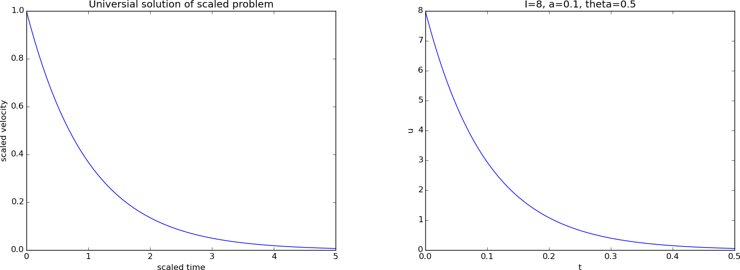
Scaled (left) and unscaled (right) exponential decay
Note that we write a message Computing the numerical solution inside
the solver_scaled function. We can then easily detect when
the solution is actually computed from scratch
and when it is simply read from file (followed by the unscaling procedure).
Here is a demo:
Terminal> # Very first run
Terminal> python decay_scaled.py --T 7 --a 1 --I 0.5 --dt 0.2
[Memory] Calling __main__--home-hpl...
solver_scaled-alias(7.0, 0.2, 0.5)
Computing the numerical solution

Terminal> # No change of T, dt, theta - can reuse solution in file
Terminal> python decay_scaled.py --T 7 --a 4 --I 2.5 --dt 0.2

Terminal> # Change of dt, must recompute
Terminal> python decay_scaled.py --T 7 --a 4 --I 2.0 --dt 0.5
[Memory] Calling __main__--home-hpl...
solver_scaled-alias(7.0, 0.5, 0.5)
Computing the numerical solution

Terminal> # Change of dt again, but dt=0.2 is already in a file
Terminal> python decay_scaled.py --T 7 --a 0.5 --I 1 --dt 0.2
We realize that joblib has access to all previous runs and does not
recompute unless it is strictly required. Our previous implementation
without joblib (in decay_scaled_v1.py)
used only one file (for one numerical case)
and will therefore perform many more calls to
solver_unscaled.
On the implementation of a simple memoize function
A memoized function recalls previous results when the same set of arguments is encountered. That is, the function caches its results. A simple implementation stores the arguments in a function call and the returned results in a dictionary, and if the arguments are seen again, one looks up in the dictionary and returns previously computed results:
class Memoize:
    def __init__(self, f):
        self.f = f
        self.memo = {}  # map arguments to results

def __call__(self, *args):
        if not args in self.memo:
            self.memo[args] = self.f(*args)
        return self.memo[args]

# Wrap my_compute_function(arg1, arg2, ...)
my_compute_function = Memoize(my_compute_function)
The memoize functionality in joblib.Memory is more sophisticated and
can work very efficiently with large array data structures as arguments.
Note that the simple version above can only be used when all arguments to
the function f are immutable (since the key in a dictionary has to be
immutable).
Scaling a generalized problem
Now we consider an extension of the exponential decay ODE to the form
One particular model, with constant \(a\) and \(b\), is a spherical small-sized organism falling in air,
where \(d\), \(\mu\), \(\varrho_b\), \(\varrho\), \(V\), and \(g\) are physical parameters. The function \(u(t)\) represents the vertical velocity, being positive upwards. We shall use this model in the following.
Exact solution
It can be handy to have the exact solution for reference, in case of constant \(a\) and \(b\):
Solving differential equations in SymPy
It can be very useful to use a symbolic computation tool such as SymPy to aid us in solving differential equations. Let us therefore demonstrate how SymPy can be used to find this solution. First we define the parameters in the problem as symbols and \(u(t)\) as a function:
>>> from sympy import *
>>> t, a, b, I = symbols('t a b I', real=True, positive=True)
>>> u = symbols('u', cls=Function)
The next task is to define the differential equation, either as
a symbolic expression that is to equal zero, or as
an equation Eq(lhs, rhs) with lhs and rhs as expressions for
the left- and right-hand side):
>>> # Define differential equation
>>> eq = diff(u(t), t) + a*u(t) - b
>>> # or
>>> eq = Eq(diff(u(t), t), -a*u(t) + b)
The differential equation can be solved by the dsolve function, yielding
an equation of the form u(t) == expression. We want to grab the
expression on the right-hand side as our solution:
>>> sol = dsolve(eq, u(t))
>>> print sol
u(t) == (b + exp(a*(C1 - t)))/a
>>> u = sol.rhs                    # grab solution
>>> print u
(b + exp(a*(C1 - t)))/a
The solution contains the unknown integration constant C1, which must
be determined by the initial condition. We form the equation arising
from the initial condition \(u(0)=I\):
>>> C1 = symbols('C1')
>>> eq = Eq(u.subs(t, 0), I)   # substitute t by 0 in u
>>> sol = solve(eq, C1)
>>> print sol
[log(I*a - b)/a]
The one solution that was found (stored in a list!)
must then be substituted back in the
expression u to yield the final solution:
>>> u = u.subs(C1, sol[0])
>>> print u
(b + exp(a*(-t + log(I*a - b)/a)))/a
As in mathematics with pen and paper, we strive to simplify expressions also in symbolic computing software. This frequently requires some trial and error process with SymPy’s simplification functions. A very standard first try is to expand everything and run simplification algorithms:
>>> u = simplify(expand(u))
>>> print u
(I*a + b*exp(a*t) - b)*exp(-a*t)/a
Doing latex(u) automatically converts the expression to LaTeX syntax
for inclusion in reports.
The reader may wonder why we bother with scaling of differential equations if SymPy can solved the problem in a nice, closed formula. This is true in the present introductory problem, but in a more general problem setting, we have some differential equation where SymPy perhaps can help with finding an exact solution only in a special case. We can use this special-case solution to control our reasoning about scales in the more general setting.
Theory
The challenges in our scaling is to find the right \(u_c\) and \(t_c\) scales. From (9) we see that if \(u'\rightarrow 0\) as \(t\rightarrow\infty\), \(u\) approaches the constant value \(b/a\). It can be convenient to let the scaled \(\bar u\rightarrow 1\) as we approach the \(d\bar u/d\bar t = 0\) state. This idea points to choosing
On the sign of the scaled velocity
A little note on the sign of \(u_c\) is necessary here. With \(\varrho_b < \varrho\), the buoyancy force upwards wins over the gravity force downwards, and the body will move upwards. In this case, the terminal velocity \(u_c > 0\). When \(\varrho_b > \varrho\), we get a motion downwards, and \(u_c < 0\). The corresponding \(u\) is then also negative, but the scaled velocity \(u/u_c\), becomes positive.
Inserting \(u = u_c\bar u = b\bar u/a\) and \(t=t_c\bar t\) in (9) leads to
We want the scales such that \(d\bar u/d\bar t\) and \(\bar u\) are about unity. To balance the size of \(\bar u\) and \(d\bar u/d\bar t\) we must therefore choose \(t_c = 1/a\), resulting in the scaled ODE problem
where \(\beta\) is a dimensionless number,
reflecting the ratio of the initial velocity and the terminal (\(t\rightarrow \infty\)) velocity \(b/a\). Scaled equations normally end up with one or more dimensionless parameters, such as \(\beta\) here, containing ratios of physical effects in the model. Many more examples on dimensionless parameters will appear in later sections.
The analytical solution of the scaled model (12) reads
The result (12) with the solution (14) is actually astonishing if \(a\) and \(b\) are as in (10): the six parameters \(d\), \(\mu\), \(\varrho_b\), \(\varrho\), \(V\), and \(g\) are conjured to one:
which is an enormous simplification of the problem if our aim is to investigate how \(u\) varies with the physical input parameters in the model. In particular, if the motion starts from rest, \(\beta=0\), and there are no physical parameters in the scaled model! We can then perform a single simulation and recover all physical cases by the unscaling procedure. More precisely, having computed \(\bar u(\bar t)\) from (12), we can use
to scale back to the original
problem again.
We observe that (12) can utilize a solver
for (9) by setting \(a=1\), \(b=1\), and \(I=\beta\).
Given some implementation of a solver for (9),
say solver(I, a, b, T, dt, theta),
the scaled model is run by solver(beta, 1, 1, T, dt, theta).
Software
We may develop a solver for the scaled problem that uses joblib
to cache solutions with the same \(\beta\), \(\Delta t\), and \(T\).
For now we fix \(\theta=0.5\).
The module decay_vc.py
(see the
section Implementation of the generalized model problem
[Ref07] for details)
has a function
solver(I, a, b, T, dt, theta) for solving \(u'(t)=-a(t)u(t)+b(t)\) for
\(t\in (0,T]\), \(u(0)=I\), with time step dt.
We reuse this function and call it with \(a=b=1\) and \(I=\beta\) to solve
the scaled problem:
from decay_vc import solver as solver_unscaled

def solver_scaled(beta, T, dt, theta=0.5):
    """
    Solve u'=-u+1, u(0)=beta for (0,T]
    with step dt and theta method.
    """
    print 'Computing the numerical solution'
    return solver_unscaled(
        I=beta, a=lambda t: 1, b=lambda t: 1,
        T=T, dt=dt, theta=theta)

import joblib
disk_memory = joblib.Memory(cachedir='temp')
solver_scaled = disk_memory.cache(solver_scaled)
If we want to plot the physical solution, we need an unscale function,
def unscale(u_scaled, t_scaled, d, mu, rho, rho_b, V):
    a, b = ab(d, mu, rho, rho_b, V)
    return (b/a)*u_scaled, a*t_scaled

def ab(d, mu, rho, rho_b, V):
    g = 9.81
    a = 3*pi*d*mu/(rho_b*V)
    b = g*(rho/rho_b - 1)
    return a, b
Looking at droplets of water in air, we can fix some of the parameters
and let the size parameter \(d\) be the one for experimentation.
The following function sets physical parameters, computes \(\beta\),
runs the solver for the scaled problem (joblib detects
if it is necessary), and finally plots the scaled curve
\(\bar u(\bar t)\) and the unscaled curve \(u(t)\).
def main(dt=0.075, # Time step, scaled problem
         T=7.5,    # Final time, scaled problem
         d=0.001,  # Diameter (unscaled problem)
         I=0,      # Initial velocity (unscaled problem)
         ):
    # Set parameters, solve and plot
    rho = 0.00129E+3  # air
    rho_b = 1E+3      # density of water
    mu = 0.001        # viscosity of water
    # Asumme we have list or similar for d
    if not isinstance(d, (list,tuple,np.ndarray)):
        d = [d]

    legends1 = []
    legends2 = []
    plt.figure(1)
    plt.figure(2)
    betas = []     # beta values already computed (for plot)

    for d_ in d:
        V = 4*pi/3*(d_/2.)**3  # volume
        a, b = ab(d_, mu, rho, rho_b, V)
        beta = I*a/b
        # Restrict to 3 digits in beta
        beta = abs(round(beta, 3))

        print 'beta=%.3f' % beta
        u_scaled, t_scaled = solver_scaled(beta, T, dt)

        # Avoid plotting curves with the same beta value
        if not beta in betas:
            plt.figure(1)
            plt.plot(t_scaled, u_scaled)
            plt.hold('on')
            legends1.append('beta=%g' % beta)
        betas.append(beta)

        plt.figure(2)
        u, t = unscale(u_scaled, t_scaled, d_, mu, rho, rho_b, V)
        plt.plot(t, u)
        plt.hold('on')
        legends2.append('d=%g [mm]' % (d_*1000))
    plt.figure(1)
    plt.xlabel('scaled time'); plt.ylabel('scaled velocity')
    plt.legend(legends1, loc='lower right')
The most complicated part of the code is related to plotting, but this part can be skipped when trying to understand how we work with a scaled model to perform the computations. The complete program is found in the file falling_body.py.
Since \(I=0\) implies \(\beta=0\), we can run different \(d\) values without any need to recompute \(\bar u(\bar t)\) as long as we assume the particle starts from rest.
From the scaling, we see that \(u_c = b/a\sim d^{-2}\) and also that \(t_c=1/a \sim d^{-2}\), so plotting of \(u(t)\) with dimensions for various \(d\) values will involve significant variations in the time and velocity scales. Figure Velocity of falling body: scaled (left) and with dimensions (right) has an example with \(d=1,2,3\) mm, where we clearly see the different time and velocity scales in the figure with unscaled variables. Note that the scaled velocity is positive because of the sign of \(u_c\) (see the box above).
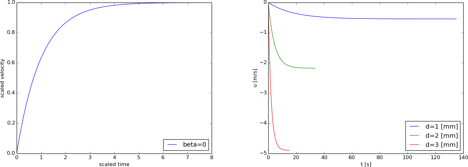
Velocity of falling body: scaled (left) and with dimensions (right)
Variable coefficients
When a prescribed coefficient like \(a(t)\) in \(u'(t) = -a(t)u(t)\) varies with time one usually also performs a scaling of this \(a\),
where the goal is to have the scaled \(\bar a\) of size unity: \(|\bar a|\leq 1\). This property is obtained by choosing \(a_c\) as the maximum value of \(|a(t)-a_0|\) for \(t\in [0,T]\), which is usually a quantity that can be estimated since \(a(t)\) is known as a function of \(t\). The \(a_0\) parameter can be chosen as 0 here. (It could be tempting to choose \(a_0=\min_t a(t)\) so that \(0\leq \bar a\leq 1\), but then there is at least one point where \(\bar a = 0\) and the differential equation collapses to \(u'=0\).)
As an example, imagine a decaying cell culture where we at time \(t_1\) change the environment (typically the nutrition) such that the death rate increases by a factor 5. Mathematically, \(a(t) = d\) for \(t < t_1\) and \(a(t)=5d\) for \(t\geq t_1\). The model reads \(u'=-a(t)u\), \(u(0)=I\).
The \(a(t)\) function is scaled by letting the characteristic size be \(a_c=d\) and \(a_0=0\):
The scaled equation becomes
The natural choice of \(u_c\) is \(I\). The characteristic time, previously taken as \(t_c=1/a\), can now be chosen as \(t_c=t_1\) or \(t_c=1/d\). With \(t_c=1/d\) we get
where
is a dimensionless number in the problem. With \(t_c=t_1\), we get
The dimensionless parameter \(\gamma\) is now in the equation rather than in the definition of \(\bar a\). Both problems involve \(\gamma\), which is the ratio between the time when the environmental change happens and the typical time for the decay (\(1/d\)).
A computation with the scaled model (16) and the original model with dimensions appears in Figure Exponential decay with jump: scaled model (left) and unscaled model (right).
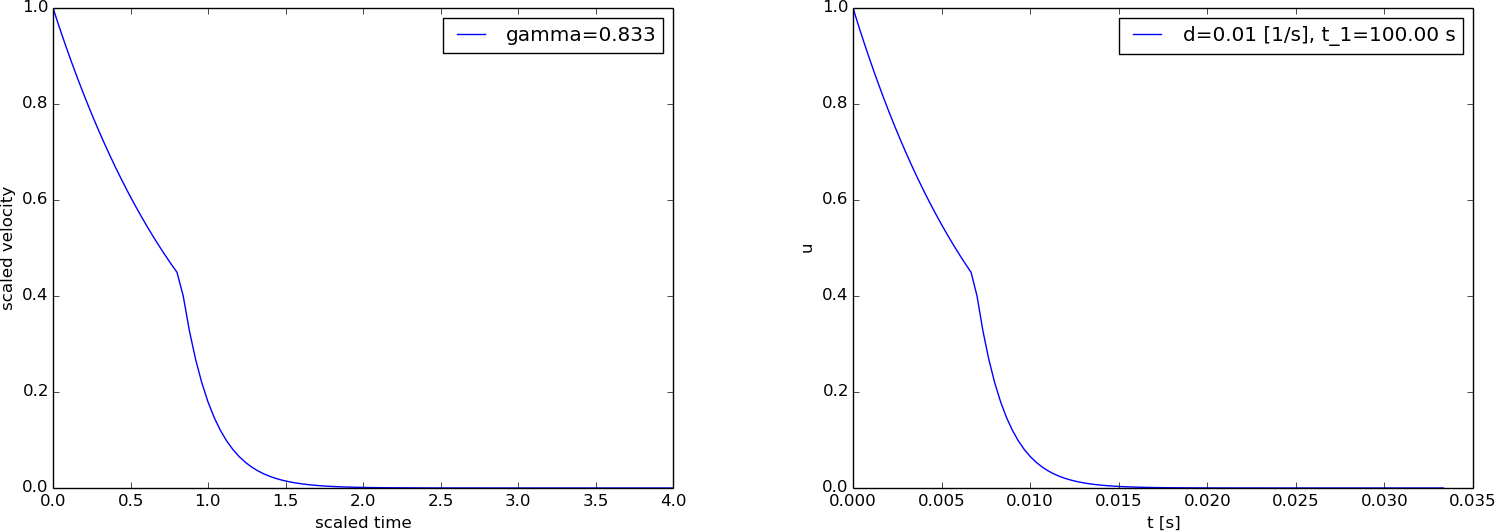
Exponential decay with jump: scaled model (left) and unscaled model (right)
Scaling a cooling problem with constant temperature in the surroundings
The heat exchange between a body at temperature \(T(t)\) and the surroundings at constant temperature \(T_s\) can be modeled by Newton’s law of cooling:
where \(k\) is a prescribed heat transfer coefficient.
Exact solution
An analytical solution is always handy to have as a control of the choice of scales. The solution of (17) is by standard methods for ODEs found to be \(T(t) = T_s + (T_0 - T_s)e^{-kt}\).
Scaling
Physically, we expect the temperature to start at \(T_0\) and then to move toward the temperature of the surroundings (\(T_s\)). We therefore expect that \(T\) lies between \(T_0\) and \(T_s\). This is mathematically demonstrated by the analytical solution as well. A proper scaling is therefore to scale and translate \(T\) according to
Now, \(0\leq \bar T\leq 1\).
Scaling time by \(\bar t = t/t_c\) and inserting \(T= T_0 + (T_s-T_0)\bar T\) and \(t=t_c\bar t\) in the problem (17) gives
A natural choice, as argued in other exponential decay problems, is to choose \(t_ck=1\), which leaves us with the scaled problem
No physical parameter enters this problem! Our scaling implies that \(\bar T\) starts at 0 and approaches 1 as \(\bar t\rightarrow\infty\), also in the case \(T_s < T_0\). The physical temperature is always recovered as
Alternative scaling
An alternative temperature scaling is to choose
Now \(\bar T=1\) initially and approaches zero as \(t\rightarrow\infty\). The resulting scaled ODE problem then becomes
with solution \(\bar T = e^{-\bar t}\).
Scaling a cooling problem with time-dependent surroundings
Let us apply the model (17) to the case when the surrounding temperature varies in time. Say we have an oscillating temperature environment according to
where \(T_m\) is the mean temperature in the surroundings, \(a\) is the amplitude of the variations around \(T_m\), and \(2\pi/\omega\) is the period of the temperature oscillations.
Exact solution
Also in this relatively simple problem it is possible to solve the differential equation problem analytically. Such a solution may be a good help to see what the scales are, and especially to control other forms for reasoning about the scales. Using the method of integrating factors for the original differential equation, we have
With \(T_s(t)=T_m + a\sin (\omega t)\) we can use SymPy to help us with
integrations (note that we use w for \(\omega\) in the computer code):
>>> from sympy import *
>>> t, k, T_m, a, w = symbols('t k T_m a w', real=True, positive=True)
>>> T_s = T_m + a*sin(w*t)
>>> I = exp(k*t)*T_s
>>> I = integrate(I, (t, 0, t))
>>> Q = k*exp(-k*t)*I
>>> Q = simplify(expand(Q))
>>> print Q
(-T_m*k**2 - T_m*w**2 + a*k*w +
(T_m*k**2 + T_m*w**2 + a*k**2*sin(t*w) -
a*k*w*cos(t*w))*exp(k*t))*exp(-k*t)/((k**2 + w**2))
Reordering the result, we get
Scaling
The scaling (18) brings in a time-dependent characteristic temperature scale \(T_s-T_0\). Let us start with a fixed scale, where we take the characteristic temperature variation to be \(T_m - T_0\):
We realize by physical reasoning that \(T\) sets out at \(T_0\), but with time, it will oscillate around \(T_m\). (This reasoning can be controlled by looking at the exact solution we produced above.) The typical average temperature span is therefore \(|T_m-T_0|\), unless \(a\) is much larger than \(|T_m-T_0|\) or \(T_0\) is very close to \(T_m\) (see Exercise 2.3: Perform alternative scalings for a discussion of these cases).
We get from the differential equation, with \(t_c=1/k\) as in the former case,
resulting in
where we have two dimensionless numbers:
The \(\alpha\) quantity measures the ratio of temperatures: amplitude of oscillations versus distance from initial temperature to the average temperature for large times. The \(\beta\) number is the ratio of the two time scales: the frequency of the oscillations in \(T_s\) and the inverse e-folding time of the heat transfer. For clear interpretation of \(\beta\) we may introduce the period \(P=2\pi/\omega\) of the oscillations in \(T_s\) and the e-folding time \(e=1/k\). Then \(\beta = 2\pi e/P\) and measures the e-folding time versus the period.
Remark
The original problem features five physical parameters: \(k\), \(T_0\), \(T_m\), \(a\), and \(\omega\), but only two dimensionless numbers appear in the scaled model (24). In fact, this is an example where application of the Pi theorem (see the section The Buckingham Pi theorem) falls short. Since, only time and temperature are involved as unit types, the theorem predicts that the five parameters yields three dimensionless numbers, not two. Scaling of the differential equations, on the other hand, shows us that the two parameters \(T_m\) and \(T_0\) affect the nature of the problem only through their difference.
Software
Implementations of the unscaled problem (17) can be reused for the scaled model by setting \(k=1\), \(T_0=0\), and \(T_s(t) = 1 + \alpha\sin (\beta \bar t)\) (\(T_m=1\), \(a=\alpha\), \(\omega =\beta\)). The file osc_cooling.py contains solvers for the problem with dimensions and for the scaled problem. The figure below shows three cases of \(\beta\) values: small, medium, and large.
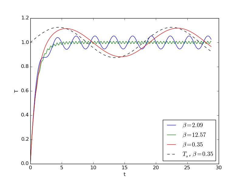
For the small \(\beta\) value, the oscillations in the surrounding temperature are slow enough compared to \(k\) for the heating and cooling process to follow the surrounding temperature, with a small time lag. For larger \(\beta\), the heating and cooling require more time, and the oscillations get smaller.
Discussion of the time scale
There are two time variations of importance in the present problem: heat is transferred to the surroundings at a rate \(k\), and the surroundings have a temperature variation with a period that goes like \(1/\omega\). (We can, when we are so lucky that we have an analytical solution at hand, inspect this solution to see that \(k\) impacts the problem through a decay factor \(e^{-kt}\), and \(\omega\) impacts the problem through oscillations \(\sin(\omega t)\).) The \(k\) parameter related to temperature decay points to a time scale \(t_c=1/k\), while the temperature oscillations of the surroundings point to a time scale \(t_c=1/\omega\). Which one should be chosen?
Bringing the temperature from \(T_0\) to the level of the surroundings, \(T_m\), goes like \(e^{-kt}\), so in this process \(t_c=1/k\) is the characteristic time. Thereafter, the body’s temperature just responds to the oscillations and the \(\sin (\omega t)\) (and \(\cos(\omega t)\)) term dominates. For these large times, \(t_c=1/\omega\) is the appropriate time scale. Choosing \(t_c=1/\omega\) results in
Let us illustrate another, less effective, scaling. The temperature scale in (18) looks natural, so we apply this choice of scale. The characteristic temperature \(T_0-T_s\) now involves a time-dependent term \(T_s(t)\). The mathematical steps become a bit more technically involved:
With \(\bar t = t/t_c = kt\) we get from the differential equation
which after dividing by \(k(T_s-T_0)\) results in
or
The last term is complicated and becomes more tractable if we factor out dimensionless numbers. To this end, we scale \(T_s\) by (e.g.) \(T_m\), which means to factor out \(T_m\) in the denominator. We are then left with
where \(\alpha\), \(\beta\), and \(\gamma\) are dimensionless numbers characterizing the relative importance of parameters in the problem:
We notice that (26) is not a special case of the original problem (17). Furthermore, the original five parameters \(k\), \(T_m\), \(a\), \(\omega\), and \(T_0\) are reduced to three dimensionless parameters. We conclude that this scaling is inferior, because using the temperature scale \(T_0-T_m\) enables reuse of the software for the unscaled problem and only two dimensionless parameters appear in the scaled model.
Let us briefly mention another possible temperature scaling: \(\bar T = T/T_m\), motivated by the fact that as \(t\rightarrow\infty\), \(T\) will oscillate around \(T_m\), so this \(\bar T\) will oscillate around unity. We get the dimensionless ODE
with a new dimensionless parameter \(\delta = a/T_m\). However, the initial condition becomes \(\bar T(0)=T_0/T_m\), and the ratio \(T_0/T_m\) is a third dimensionless parameter, so this scaling is also inferior to the one above with only two parameters.
Scaling a nonlinear ODE
Exponential growth models, \(u'=au\), are not realistic in environments with limited resources. However, by letting \(a\) depend on \(u\), the effect of limited resources can well be captured by such a simple differential equation model:
If the maximum value of \(u\) is denoted by \(M\), we have that \(a(M)=0\). A simple choice fulfilling this requirement is \(a(u)=\varrho(1-u/M)\). The parameter \(\varrho\) can be interpreted as the initial exponential growth rate if we assume that \(I/M\ll 1\), since at \(t=0\) the model then approximates \(u'=\varrho u\).
The choice \(a(u)=\varrho(1-u/M)\) is known as the logistic model for population growth:
A more complicated choice of \(a\) may be \(a(u)=\varrho(1-u/M)^p\) for some exponent \(p\) (this function also fulfills \(a(M)=0\) and \(a\approx\varrho\) for \(t=0\)).
Scaling
Let us scale (28) with \(a(u)=\varrho (1-u/M)^p\). The natural scale for \(u\) is \(M\) (\(u_c=M\)), since we know that \(0 < u\leq M\), and this makes the dimensionless \(\bar u = u/M \in (0,1]\). The function \(a(u)\) is typically varying between 0 and \(\varrho\), so it can be scaled as
Time is scaled as \(\bar t = t/t_c\) for some suitable characteristic time \(t_c\). Inserted in (28), we get
resulting in
A natural choice is \(t_c =1/\varrho\) as in other exponential growth models since it leads to the term on the right-hand side to be about unity, just as the left-hand side. (If the scaling is correct, \(\bar u\) and its derivatives are of order unity, so the coefficients must also be of order unity.) Introducing also the dimensionless parameter
measuring the fraction of the initial population compared to the maximum one, we get the dimensionless model
Here, we have two dimensionless parameters: \(\alpha\) and \(p\). A classical logistic model with \(p=1\) has only one dimensionless variable.
Alternative scaling
We could try another scaling of \(u\) where we also translate \(\bar u\):
This choice of \(\bar u\) results in
The essential difference between (30) and (31) is that \(\bar u\in [\alpha, 1]\) in the former and \(\bar u \in [0, 1-\alpha]\) in the latter. Both models involve the dimensionless numbers \(\alpha\) and \(p\). An advantage of (30) is that software for the unscaled model can easily be used for the scaled model by choosing \(I=\alpha\), \(M=1\), and \(\varrho=1\).
SIR ODE system for spreading of diseases
The field of epidemiology frequently applies ODE systems to describe the spreading of diseases, such as smallpox, measles, plague, ordinary flu, swine flu, and HIV. Different models include different effects, which are reflected in dimensionless numbers. Most of the effects are modeled as exponential decay or growth of the dependent variables.
The simplest model has three categories of people: susceptibles (S) who can get the disease, infectious (I) who are infected and may infect susceptibles, and recovered (R) who have recovered from the disease and gained immunity. We introduce \(S(t)\), \(I(t)\), and \(R(t)\) as the number of people in the categories S, I, and R, respectively. The model, naturally known as the SIR model, can be expressed as a system of three ODEs:
where \(\beta\) and \(\nu\) are empirical constants. The average time for recovering from the disease can be shown to be \(\nu^{-1}\), but \(\beta\) is much harder to estimate, so working with a scaled model where \(\beta\) is “scaled away” is advantageous.
Scaling
It is natural to scale \(S\), \(I\), and \(R\) by, e.g., \(S(0)\):
Introducing \(\bar t = t/t_c\), we arrive at the equations
with initial conditions \(\bar S(0)=1\), \(\bar I(0)=I_0/S(0)=\alpha\), and \(\bar R(0)=R(0)/S(0)\). Normally, \(R(0)=0\).
Taking \(t_c=1/\nu\), corresponding to a time unit equal to the time it takes to recover from the disease, we end up with the scaled model
with \(\bar S(0)=1\), \(\bar I(0)=\alpha\), \(\bar R(0)=0\), and \(R_0\) as the dimensionless number
We see from (36) that to make the disease spreading, \(d\bar I/d\bar t >0\), and therefore \(R_0 \bar S(0) - 1 > 0\) or \(R_0 > 1\) since \(\bar S(0)=1\). Therefore, \(R_0\) reflects the disease’s ability to spread and is consequently an important dimensionless quantity, known as the basic reproduction number. This number reflects the number of infected people caused by one infectious individual during the time period of the disease.
Looking at (33), we see that to increase \(I\) initially, we must have \(dI/dt >0\) at \(t=0\), which implies \(\beta I(0)S(0) - \nu I(0) >0\), i.e., \(R_0 > 1\).
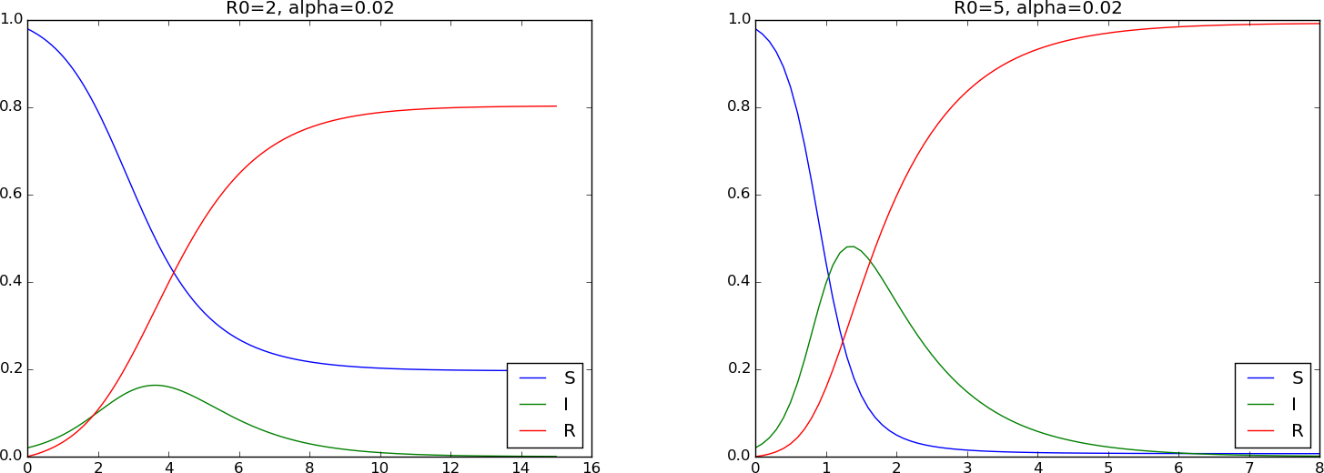
Software
Any implementation of the SIR model with dimensions can be reused for the scaled model by setting \(\beta = R_0\), \(\nu = 1\), \(S(0)=1-\alpha\), and \(I(0)=\alpha\). Below is a plot with two cases: \(R_0=2\) and \(R_0=5\), both with \(\alpha=0.02\).
Alternative scaling
where \(N\) is the size of the population. We can therefore scale \(S\), \(I\), and \(R\) by the total population \(N=S(0)+I(0)+R(0)\):
With the same time scale, one gets the system (35)-(37), but with \(R_0\) replaced by the dimensionless number:
The initial conditions become \(\bar S(0)=1-\alpha\), \(\bar I(0)=\alpha\), and \(\bar R(0)=0\).
For the disease to spread at \(t=0\), we must have \(\tilde R_0 \bar S(0) > 1\), but \(\tilde R_0 \bar S(0) = N\beta/\nu \cdot S(0)/N = R_0\), so the criterion is still \(R_0 > 1\). Since \(R_0\) is a more famous number than \(\tilde R_0\), we can write the ODEs with \(R_0/S(0) = R_0/(1-\alpha)\) instead of \(\tilde R_0\).
Choosing \(t_c\) to make the \(SI\) terms balance the time derivatives, \(t_c = (N\beta)^{-1}\), moves \(\tilde R_0\) (or \(R_0\) if we scale \(S\), \(I\), and \(R\) by \(S(0)\)) to the \(I\) terms:
SIRV model with finite immunity
A common extension of the SIR model involves finite immunity: after some period of time, recovered individuals lose their immunity and become susceptibles again. This is modeled as a leakage \(-\mu R\) from the R to the S category, where \(\mu^{-1}\) is the average time it takes to lose immunity. Vaccination is another extension: a fraction \(pS\) is removed from the S category by successful vaccination and brought to a new category V (the vaccinated). The ODE model reads
Using \(t_c=1/\nu\) and scaling the unknowns by \(S(0)\), we arrive at the dimensionless model
with two new dimensionless parameters:
The quantity \(p^{-1}\) can be interpreted as the average time it takes to vaccinate a susceptible successfully. Writing \(\gamma = \nu^{-1}/\mu^{-1}\) and \(\delta = \nu^{-1}/p^{-1}\) gives the interpretation that \(\gamma\) is the ratio of the average time to recover and the average time to lose immunity, while \(\delta\) is the ratio of the average time to recover and the average time to successfully vaccinate a susceptible.
The plot in Figure Spreading of a disease with loss of immunity (left) and added vaccination (right) has \(\gamma = 0.05\), i.e., loss of immunity takes 20 weeks if it takes one week to recover from the disease. The left plot corresponds to no vaccination, while the right has \(\delta = 0.5\) for a vaccination campaign that lasts from day 7 to day 15. The value \(\delta =0.5\) reflects that it takes two weeks to successfully vaccinate a susceptible, but the effect of vaccination is still dramatic.
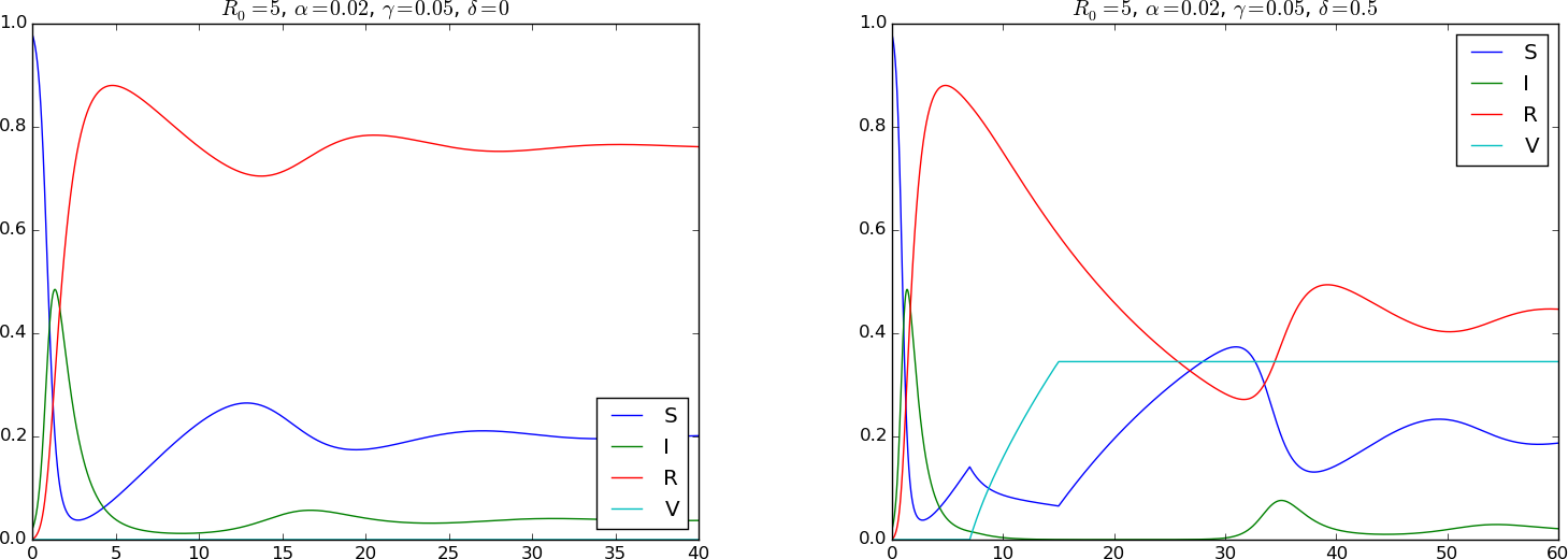
Spreading of a disease with loss of immunity (left) and added vaccination (right)
Michaelis-Menten kinetics for biochemical reactions
A classical reaction model in biochemistry describes how a substrate S is turned into a product P with aid of an enzyme E. S and E react to form a complex ES in the first stage of the reaction. In the second stage, ES is turned into E and P. Introducing the amount of S, E, ES, and P by \([S]\), \([E]\), \([ES]\), and \([P]\), the mathematical model can be written as
The initial conditions are \([ES](0)=[P](0)=0\), and \([S]=S_0\), \([E]=E_0\). Three rate constants are involved: \(k_+\), \(k_-\), and \(k_v\). The above mathematical model is known as Michaelis-Menten kinetics.
The amount of substance is measured in the unit mole (mol). From the equations we can see that \(k_+\) is measured in \(\hbox{s}^{-1}\hbox{mol}^{-1}\), while \(k_-\) and \(k_v\) are measured in \(\hbox{s}^{-1}\). It is convenient to get rid of the mole unit for the amount of a substance. When working with dimensionless quantities, only ratios of the rate constants and not their specific values are needed.
Classical analysis
A common assumption is that the formation of \([ES]\) is very fast and that it quickly reaches an equilibrium state, \([ES]^{\prime}=0\). Equation (48) then reduces to the algebraic equation
which leads to
where \(K\) is the famous Michaelis constant - the equilibrium constant between \([E][S]\) and \([ES]\).
Another important observation is that the ODE system implies two conservation equations, arising from simply adding the ODEs:
from which it follows that
We can use (55) and (52) to express \([E]\) by \([S]\):
Now (50) can be developed to an equation involving \([S]\) only:
We see that the parameter \(K\) is central.
From above expression for \([E]\) and (55) it now follows
If \(K\) is comparable to \(S_0\) these indicate
as is used for scaling \([E]\) and \(Q_c\), subsequently. Provided we exclude the case \([S]\gg K\), we may infer that \([E]\) will be of magnitude \(E_0\), while \([ES]\) will be of magnitude \(E_0 S_0/K\).
Dimensionless ODE system
Let us reason how to make the original ODE system (48)-(51) dimensionless. Aiming at \([S]\) and \([E]\) of unit size, two obvious dimensionless unknowns are
For the other two unknowns we just introduce scales to be determined later:
With \(\bar t = t/t_c\) the equations become
Determining scales
Choosing the scales is actually a quite complicated matter that requires extensive analysis of the equations to determine the characteristics of the solutions. Much literature is written about this, but here we shall take a simplistic and pragmatic approach. Besides the Michaelis constant \(K\), there is another important parameter,
because most applications will involve a small \(\epsilon\). We shall have \(K\) and \(\epsilon\) in mind while choosing scales such that these symbols appear naturally in the scaled equations.
Looking at the equations, we see that the \(K\) parameter will appear if \(t_c\sim 1/k_+\). However, \(1/k_+\) does not have the dimension \(\hbox{[T]}^{-1}\) as required, so we need to add a factor with dimension mol. A natural choice is \(t_c^{-1}=k_+S_0\) or \(t_c^{-1}=k_+E_0\). Since often \(S_0\gg E_0\), the former \(t_c\) is a short time scale and the latter is a long time scale. If the interest is in the long time scale, we set
The equations then take the form
The \([ES]\) variable starts and ends at zero, and its maximum value can be roughly estimated from the equation for \([ES]^\prime\) by setting \([ES]^\prime = 0\), which gives
where we have replaced \([E][S]\) by \(E_0S_0\) as an identification of magnitude. This magnitude of \([ES]\) at its maximum can be used as the characteristic size \(Q_c\):
The equation for \(\bar P\) simplifies if we choose \(P_c=Q_c\). With these assumptions one gets
We can now identify the dimensionless numbers
where we see that \(\alpha = \beta + \gamma\), so \(\gamma\) can be eliminated. Moreover,
implying that \(\alpha > \beta\).
We arrive at the final set of scaled differential equations:
The initial conditions are \(\bar S=\bar E =1\) and \(\bar Q=\bar P=0\).
The five initial parameters (\(S_0\), \(E_0\), \(k_+\), \(k_-\), and \(k_v\)) are reduced to three dimensionless constants:
- \(\alpha\) is the dimensionless Michaelis constant, reflecting the ratio of the production of P and E (\(k_v+k_-\)) versus the production of the complex (\(k_+\)), made dimensionless by \(E_0\),
- \(\epsilon\) is the initial fraction of enzyme relative to the substrate,
- \(\beta\) measures the relative importance of production of P (\(k_v\)) versus production of the complex (\(k_+\)), made dimensionless by \(E_0\).
Observe that software developed for solving (48)-(51) cannot be reused for solving (58)-(61) since the latter system has a slightly different structure.
Conservation equations
The counterpart to the conservation equations (55)-(56) is obtained by adding (58) and \(\alpha\) times (61), and adding (58), (59), and \(\alpha\) times (60):
The scaled quantities, as well as the original concentrations, must be positive variables, and \(\bar E\in [0,1]\), \(\bar S\in [0,1]\). Such checks along with the conserved quantities above should be performed at every time step in a simulation.
Analysis of the scaled system
In the scaled system, we may assume \(\epsilon\) small, which from (61) gives rise to the simplification \(\epsilon\bar E^{\prime}=0\), and thereby the relation \(\bar Q = \bar E\bar S\). The conservation equation \([ES] + [E]= E_0\) reads \(Q_c\bar Q + E_0\bar E = E_0\) such that \(\bar E = 1 - Q_c\bar Q/E_0=1- \bar Q S_0/K = 1 - \epsilon^{-1}\alpha^{-1}\bar Q\). The relation \(\bar Q=\bar E\bar S\) then becomes
which can be solved for \(\bar Q\):
The equation (60) for \(\bar S\) becomes
This is a more precise analysis than the one leading to (57) since we now realize that the mathematical assumption for the simplification is \(\epsilon\rightarrow 0\).
Is (64) consistent with (57)? It is easy to make algebraic mistakes when deriving scaled equations, so it is always wise to carry out consistency checks. Introducing dimensions in (64) leads to
and hence with \(t_c^{-1}=k_+E_0\),
which is (57).
Figure Simulation of a biochemical process shows the impact of \(\epsilon\): with a moderately small
value (0.1) we see that \(\bar Q\approx 0\), which justifies the
simplifications performed above. We also observe that all the unknowns
vary between 0 and about 1, indicating that the scaling is successful
for the chosen dimensionless numbers. The simulations made use of
a time step \(\Delta\bar t=0.01\) with a 4th-order Runge-Kutta method,
using \(\alpha=1.5\), \(\beta=1\) (relevant code is in the
simulate_biochemical_process function in session.py).
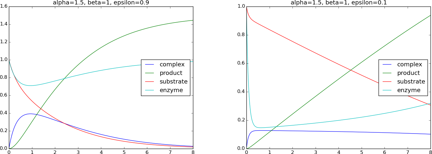
Simulation of a biochemical process
However, it is of interest to investigate the limit \(\epsilon\rightarrow 0\). Initially, the equation for \(d\bar E/d\bar t\) reads \(d\bar E/d\bar t = -\epsilon^{-1}\), which implies a very fast reduction of \(\bar E\). Using \(\epsilon=0.005\) and \(\Delta\bar t = 10^{-3}\), simulation results show that \(\bar E\) decays to approximately zero at \(t=0.03\) while \(\bar S\approx 1\) and \(\bar Q \approx \bar P\approx 0\). This is reasonable since with very little enzyme in comparison with the substrate (\(\epsilon\rightarrow 0\)) very little will happen.
Vibration problems
We shall in this section address a range of different second-order ODEs for mechanical vibrations and demonstrate how to reason about the scaling in different physical scenarios.
Undamped vibrations without forcing
The simplest differential equation model for mechanical vibrations reads
where unknown \(u(t)\) measures the displacement of the body, This is a common model for a vibrating body with mass \(m\) attached to a linear spring with spring constant \(k\) (and force \(-ku\)). Figure Oscillating body attached to a spring shows a typical mechanical sketch of such a system: some mass can move horizontally without friction and is connected to a spring that exerts a force \(-ku\) on the body.
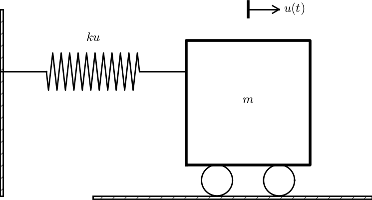
Oscillating body attached to a spring
The first technical steps of scaling
The problem (65) has one independent variable \(t\) and one dependent variable \(u\). We introduce dimensionless versions of these variables:
where \(u_c\) and \(t_c\) are characteristic values of \(u\) and \(t\). Inserted in (65), we get
resulting in
What is an appropriate displacement scale \(u_c\)? The initial condition \(u(0)=I\) is a candidate, i.e., \(u_c=I\). But how to choose the time scale? Making the coefficient in front of the \(\bar u\) unity, such that both terms balance and are of size unity, is a candidate.
The exact solution
To better see what the proper scales of \(u\) and \(t\) are, we can look into the analytical solution of this problem. Although the exact solution of (65) is quite straightforward to calculate by hand, we take the opportunity to make use of SymPy to find \(u(t)\). The use of SymPy can later be generalized to vibration ODEs that are harder to solve by hand.
SymPy requires all mathematical symbols to be explicitly created:
from sympy import *
u = symbols('u', cls=Function)
w = symbols('w', real=True, positive=True)
I, V, C1, C2 = symbols('I V C1 C2', real=True)
To specify the ODE to be solved, we can make a Python function returning all the terms in the ODE:
# Define differential equation: u'' + w**2*u = 0
def ode(u):
    return diff(u, t, t) + w**2*u

diffeq = ode(u(t))
The diffeq variable, defining the ODE, can be passed to the SymPy
function dsolve to find the symbolic solution of the ODE:
s = dsolve(diffeq, u(t))
# s is an u(t) == expression (Eq obj.), s.rhs grabs the expression
u_sol = s.rhs
print u_sol
The solution that gets printed is C1*sin(t*w) + C2*cos(t*w), indicating
that there are two integration constants C1 and C2 to be determined
by the initial conditions. The result of applying these conditions is
a \(2\times 2\) linear system of algebraic equations that SymPy can solve
by the solve function. The code goes as follows:
# The solution u_sol contains integration constants C1 and C2
# but these are not symbols, substitute them by symbols
u_sol = u_sol.subs('C1', C1).subs('C2', C2)

# Determine C1 and C2 from the initial conditions
ic = [u_sol.subs(t, 0) - I, u_sol.diff(t).subs(t, 0) - V]
print ic   # 2x2 algebraic system for C1 and C2
s = solve(ic, [C1, C2])
# s is now a dictionary: {C2: I, C1: V/w}
# substitute solution back in u_sol
u_sol = u_sol.subs(C1, s[C1]).subs(C2, s[C2])
print u_sol
The u_sol variable is now I*cos(t*w) + V*sin(t*w)/w.
Since symbolic software is far from bug-free and can give wrong results,
we should always check the answer. Here, we insert the solution in the ODE
to see if the result is zero, and we insert the solution in the initial
conditions to see that these are fulfilled:
# Check that the solution fulfills the ODE and init.cond.
print simplify(ode(u_sol)),
print u_sol.subs(t, 0) - I, diff(u_sol, t).subs(t, 0) - V
There will be many more examples on using SymPy to find exact solutions of differential equation problems.
The solution of the ODE in mathematical notation is
More insight arises from rewriting such an expression in the form \(A\cos(wt - \phi)\):
Now we see that the \(u\) corresponds to cosine oscillations with a frequency shift \(\phi\) and amplitude \(\sqrt{I^2 + (V/\omega)^2}\).
The forthcoming text relies on a good understanding of concepts like period, frequency, and amplitude of oscillating signals, so readers who need to refresh these concepts are recommended to do Problem 2.12: Find the period of sinusoidal signals before continuing.
Discussion of the displacement scale
The amplitude of \(u\) is \(\sqrt{I^2 + V^2/\omega^2}\), and this expression is obviously a candidate for \(u_c\). However, the simpler choice \(u_c=\max (I, V/\omega)\) is also relevant and more attractive than the square root expression (but potentially a factor 1.4 wrong compared to the exact amplitude). It is not very important to have \(|u|\leq 1\), the point is to avoid \(|u|\) very small or large.
Discussion of the time scale
What is an appropriate time scale? Looking at (66) and arguing that \(\bar u''\) and \(\bar u\) both should be around unity in size, the coefficient \(t_c^2k/m\) must equal unity, implying that \(t_c=\sqrt{m/k}\). Also from the analytical solution we see that the solution goes like the sine or cosine of \(\omega t\), so \(1/\omega = \sqrt{m/k}\) can be a characteristic time scale. Likewise, one period of the oscillations, \(P=2\pi/\omega\), can be the characteristic time, leading to \(t_c=2\pi/\omega\).
The dimensionless solution
With \(u_c=I\) and \(t_c=\sqrt{m/k}\) we get the scaled model
where \(\alpha\) is a dimensionless parameter:
Note that in case \(V=0\), we have “scaled away” all physical parameters. The universal solution without physical parameters is then \(\bar u(\bar t)=\cos\bar t\).
The unscaled solution is recovered as
This expressions shows that the scaling is simply a matter of stretching or shrinking the axes.
Alternative displacement scale
Using \(u_c = V/\omega\), the equation is not changed, but the initial conditions become
With \(u_c=V/\omega\) and one period as time scale, \(t_c=2\pi\sqrt{m/k}\), we get the alternative model
The unscaled solution is in this case recovered by
About frequency and dimensions
The solution goes like \(\cos\omega t\), where \(\omega =\sqrt{m/k}\) must have dimension 1/s. Actually, \(\omega\) has dimension radians per second: rad/s. A radian is dimensionless since it is arc (length) divided by radius (length), but still regarded as a unit. The period \(P\) of vibrations is a more intuitive quantity than the frequency \(\omega\). The relation between \(P\) and \(\omega\) is \(P=2\pi/\omega\). The number of oscillation cycles per period, \(f\), is a more intuitive measurement of frequency and also known as frequency. Therefore, to be precise, \(\omega\) should be named angular frequency. The relation between \(f\) and \(T\) is \(f=1/T\), so \(f=2\pi\omega\) and measured in Hz (1/s), which is the unit for counts per unit time.
Undamped vibrations with constant forcing
For vertical vibrations in the gravity field, the model (65) must also take the gravity force \(-mg\) into account:
How does the new term \(-mg\) influence the scaling? We observe that if there is no movement of the body, \(u''=0\), and the spring elongation matches the gravity force: \(ku = -mg\), leading to a steady displacement \(u=-mg/k\). We can then have oscillations around this equilibrium point. A natural scaling for \(u\) is therefore
The scaled differential equation with the same time scale as before reads
leading to
The initial conditions \(u(0)=I\) and \(u'(0)=V\) become, with \(u_c=I\),
We see that the oscillations around the equilibrium point in the gravity field are identical to the horizontal oscillations without gravity, except for an offset \(mg/(kI)\) in the displacement.
Undamped vibrations with time-dependent forcing
Now we add a transient forcing term \(F(t)\) to the model (65):
Take the forcing to be oscillating:
The technical steps of the scaling are still the same, with the intermediate result
What are typical displacement and time scales? This is not so obvious without knowing the details of the solution, because there are three parameters (\(I\), \(V\), and \(A\)) that influence the magnitude of \(u\). Moreover, there are two time scales, one for the free vibrations of the systems and one for the forced vibrations \(F(t)\).
Investigating scales via analytical solutions
As we have seen already several times, having access to
an exact solution is very fortunate as it allows us to directly
examine the scales. Also in the present problem it is possible
to derive an exact solution. We
continue the SymPy session from the previous section and perform much
of the same steps. Note that we use w for \(\omega = \sqrt{k/m}\)
in the computer code (to obtain a more direct visual counterpart to
\(\omega\)).
SymPy may get confused when coefficients in differential equations
contain several symbols. We therefore rewrite the equation with
at most one symbol in each coefficient (i.e., symbolic software is
in general
more successful when applied to scaled differential equations than the
unscaled counterparts, but right now our task is to solve the unscaled version).
The amplitude \(A/m\) in the forcing term is of this reason
replaced by the symbol A1.
A, A1, m, psi = symbols('A A1 m psi', positive=True, real=True)
def ode(u):
    return diff(u, t, t) + w**2*u - A1*cos(psi*t)

diffeq = ode(u(t))
u_sol = dsolve(diffeq, u(t))
u_sol = u_sol.rhs

# Determine the constants C1 and C2 in u_sol
# (first substitute our own declared C1 and C2 symbols,
# then use the initial conditions)
u_sol = u_sol.subs('C1', C1).subs('C2', C2)
eqs = [u_sol.subs(t, 0) - I, u_sol.diff(t).subs(t, 0) - V]
s = solve(eqs, [C1, C2])
u_sol = u_sol.subs(C1, s[C1]).subs(C2, s[C2])

# Check that the solution fulfills the equation and init.cond.
print simplify(ode(u_sol))
print simplify(u_sol.subs(t, 0) - I)
print simplify(diff(u_sol, t).subs(t, 0) - V)

u_sol = simplify(expand(u_sol.subs(A1, A/m)))
print u_sol
The output from the last line is
A/m*cos(psi*t)/(-psi**2 + w**2) + V*sin(t*w)/w +
(A/m + I*psi**2 - I*w**2)*cos(t*w)/(psi**2 - w**2)
With a bit of rewrite this expression becomes
Obviously, this expression is only meaningful for \(\psi\neq\omega\). The case \(\psi = \omega\) gives an infinite amplitude in this model, a phenomenon known as resonance. The amplitude becomes finite when damping is included, see the section Damped vibrations with forcing.
When the system starts from rest, \(I=V=0\), and the forcing is the only driving mechanism, we can simplify:
To gain more insight, \(\cos(\psi t) - \cos(\omega t)\) can be rewritten in terms of the mean frequency \((\psi + \omega)/2\) and the difference in frequency \((\psi - \omega)/2\):
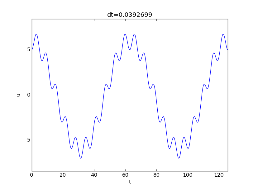
showing that there is a signal with frequency \((\psi + \omega)/2\) whose amplitude has a (much) slower frequency \((\psi - \omega)/2\). Figure Signal with frequency 3.1 and envelope frequency 0.2 shows an example on such a signal.
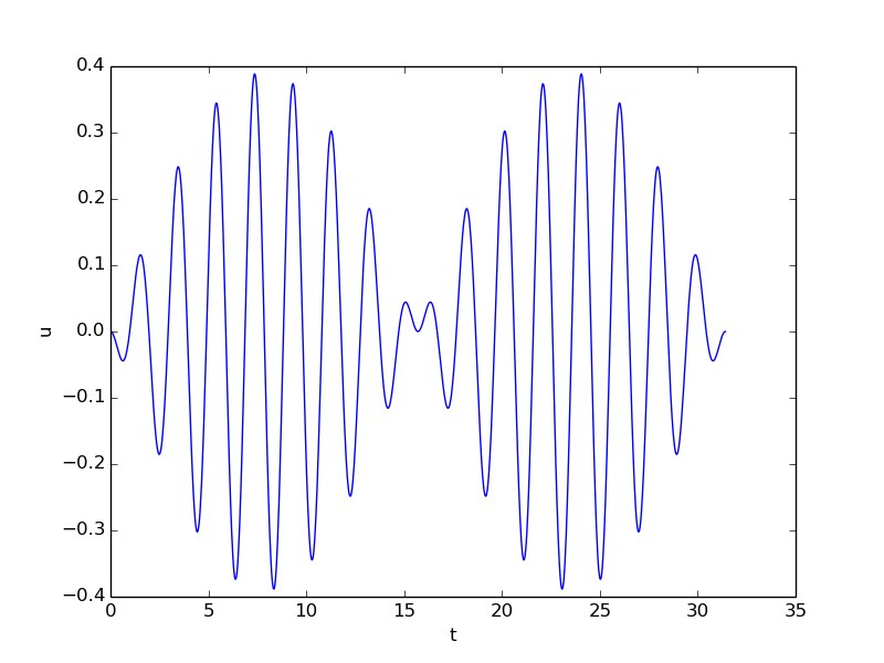
Signal with frequency 3.1 and envelope frequency 0.2
The displacement and time scales
A characteristic displacement can in the latter special case be taken as \(u_c= A/(m(\omega^2 - \psi^2))\). This is also a relevant choice in the more general case \(I\neq0, V\neq 0\), unless \(I\) or \(V\) is so large that it dominates over the amplitude caused by the forcing. With \(u_c= A/(m(\omega^2 - \psi^2))\) we also have three special cases: \(\omega \ll \psi\), \(\omega \gg\psi\), and \(\psi \sim \omega\). In the latter case we need \(u_c= A/(m(\omega^2 - \psi^2))\) if we want \(|u|\leq 1\). When \(\omega\) and \(\psi\) are significantly different, we may choose one of them and neglect the smaller. Choosing \(\omega\) means \(u_c=A/k\), which is the relevant scale if \(\omega\gg\psi\). In the opposite case, \(\omega\ll\psi\), \(u_c=A/(m\psi^2)\).
The time scale is dominated by the fastest oscillations, which are of frequency \(\psi\) or \(\omega\) when these are close and the largest of them when they are distant. In any case, we set \(t_c=1/\max(\psi,\omega)\).
Finding the displacement scale from the differential equation
Going back to (72), we may demand that all the three terms in the differential equation are of size unity. This leads to \(t_c=\sqrt{m/k}\) and \(u_c=At_c^2/m = A/k\). The formula for \(u_c\) is a kind of measure of the ratio of the forcing and the spring force (the dimensionless number \(A/(ku_c)\) would be this ratio).
Looking at (73), we see that if \(\psi\ll\omega\), the amplitude can be approximated by \(A/(m\omega^2)=A/k\), showing that the scale \(u_c=A/k\) is relevant for an excitation frequency \(\psi\) that is small compared to the free vibration frequency \(\omega\).
Scaling with free vibrations as time scale
The next step is to work out the dimensionless ODE for the chosen scales. We first select the time scale based on the free oscillations with frequency \(\omega\), i.e., \(t_c=1/\omega\). Inserting the expression in (72) results in
Here we have four dimensionless variables
We remark that the choice of \(u_c\) has so far not been made. Several different cases will be considered below, and we will see that certain choices reduce the number of independent dimensionless variables to three.
The four dimensionless variables above have interpretations as ratios of physical effects:
- \(\alpha\): ratio of the initial displacement and the characteristic response \(u_c\),
- \(\beta\): ratio of the initial velocity and the typical velocity measure \(u_c/t_c\),
- \(\gamma\): ratio of the forcing \(A\) and the mass times acceleration \(mu_c/t_c^2\) or the ratio of the forcing and the spring force \(ku_c\)
- \(\delta\): ratio of the frequencies or the time scales of the forcing and the free vibrations.
Software
Any solver for (72) can be used for (74). More details are provided at the end of the section Damped vibrations with forcing.
Choice of \(u_c\) close to resonance
Now we shall discuss various choices of \(u_c\). Close to resonance, when \(\psi\sim\omega\), we may set \(u_c=A/(m(\omega^2 - \psi^2))\). The dimensionless numbers become in this case
With \(\psi = 0.99\omega\), \(\delta =0.99\), \(V=0\), \(\alpha = \gamma = 1-\delta^2 = 0.02\), we have the problem
This is a problem with a very small initial condition and a very small forcing, but the state close to resonance brings the amplitude up to about unity, see the result of numerical simulations with \(\delta=0.99\) in Figure Forced undamped vibrations close to resonance. Neglecting \(\alpha\), the solution is given by (73), which here means \(A=1-\delta^2\), \(m=1\), \(\omega=1\), \(\psi=\delta\):
Note that this is a problem which demands very high accuracy in the numerical calculations. Using 20 time steps per period gives a significant angular frequency error and an amplitude of about 1.4. We used 160 steps per period for the results in Figure Forced undamped vibrations close to resonance.
Forced undamped vibrations close to resonance
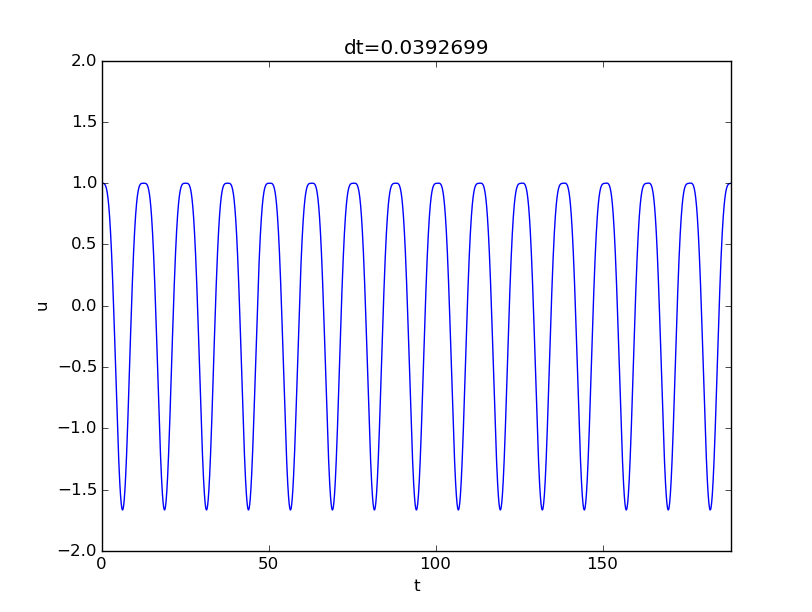
Unit size of all terms in the ODE
Using the displacement scale \(u_c=A/k\) leads to (74) with
Simulating a case with \(\delta=0.5\), \(\alpha=1\), and \(\beta=0\) gives the oscillations in Figure Forced undamped vibrations away from resonance, which is a case away from resonance, and the amplitude is about unity. However, choosing \(\delta =0.99\) (close to resonance) results in a figure similar to Figure Forced undamped vibrations close to resonance, except that the amplitude is about \(10^2\) because of the moderate size of \(u_c\). The present scaling is therefore most suitable away from resonance, and when the terms containing \(\cos\omega t\) and \(\sin\omega t\) are important (e.g., \(\omega\gg\psi\)).
Forced undamped vibrations away from resonance
Choice of \(u_c\) when \(\psi\gg\omega\)
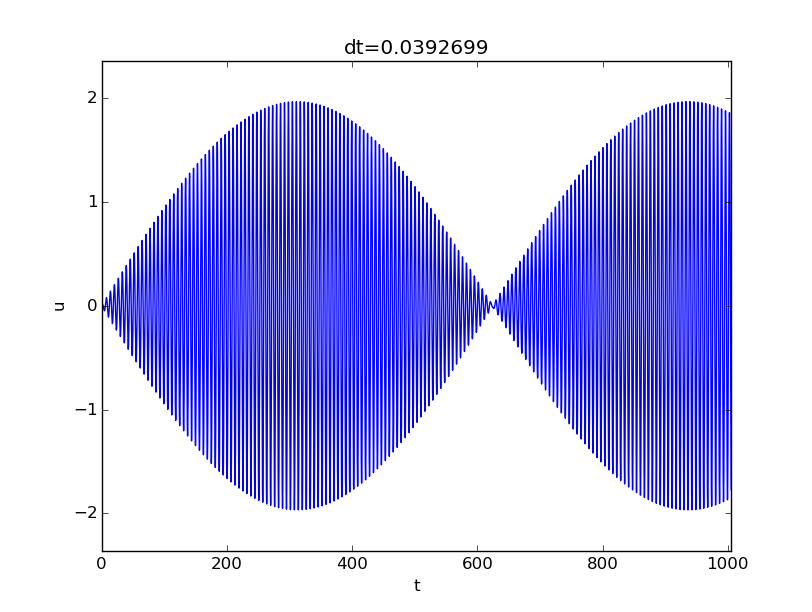
Finally, we may look at the case where \(\psi\gg\omega\) such that \(u_c=A/(m\psi^2)\) is a relevant scale (i.e., omitting \(\omega^2\) compared to \(\psi^2\) in the denominator), but in this case we should use \(t_c=1/\psi\) since the force varies much faster than the free vibrations of the system. This choice of \(t_c\) changes the scaled ODE to
where
In the regime \(\psi\gg\omega\), \(\delta\gg 1\), thus making \(\alpha\) and \(\beta\) large. However, if \(\alpha\) and/or \(\beta\) is large, the initial condition dominates over the forcing, and will also dominate the amplitude of \(u\), thereby making the scaling of \(u\) inappropriate. In case \(I=V=0\) so that \(\alpha=\beta=0\), (73) predicts (\(A=m=1\), \(\omega=\delta^{-1}\), \(\psi=1\))
which has an amplitude about \(2\) for \(\delta\gg 1\). Figure Forced undamped vibrations with rapid forcing shows a case.
Forced undamped vibrations with rapid forcing
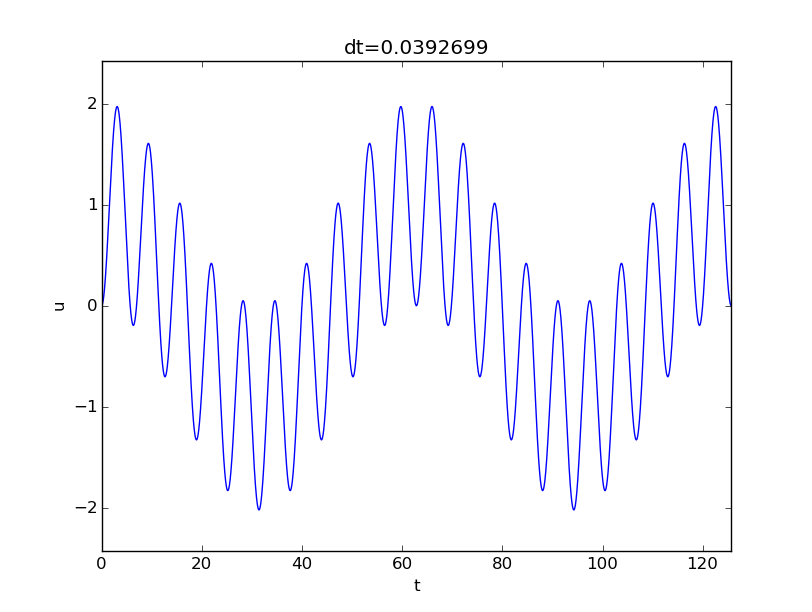
With \(\alpha=0.05\delta^2=5\), we get a significant contribution from the free vibrations (the homogeneous solution of the ODE) as shown in Figure Forced undamped vibrations with rapid forcing and initial displacement of 5. For larger \(\alpha\) values, one must base \(u_c\) on \(I\) instead. (The graphs in Figure Forced undamped vibrations with rapid forcing and Forced undamped vibrations with rapid forcing and initial displacement of 5 were produced by numerical simulations with 160 time steps per period of the forcing.)
Forced undamped vibrations with rapid forcing and initial displacement of 5
Displacement scale based on \(I\)
Choosing \(u_c=I\) gives
with
This scaling is not relevant close to resonance since then \(u_c\gg I\).
Damped vibrations with forcing
We now introduce a linear damping force \(bu'(t)\) in the equation of motion:
Figure Oscillating body with external force, attached to a spring and damper shows a typical one-degree-of-freedom mechanical system with a linear dashpot, representing the damper (\(bu'\)), a linear spring (\(ku\)), and an external force (\(F\)).
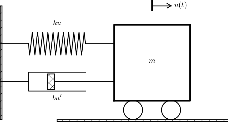
Oscillating body with external force, attached to a spring and damper
The standard scaling procedure results in
The exact solution
As always, it is a great advantage to look into exact solutions for controlling our choice of scales. Using SymPy to solve (83) is, in principle, very straightforward:
>>> diffeq = diff(u(t), t, t) + b/m*diff(u(t), t) + w**2*u(t)
>>> s = dsolve(diffeq, u(t))
>>> s.rhs
C1*exp(t*(-b - sqrt(b - 2*m*w)*sqrt(b + 2*m*w))/(2*m)) +
C2*exp(t*(-b + sqrt(b - 2*m*w)*sqrt(b + 2*m*w))/(2*m))
This is indeed the correct solution, but it is on a complex
exponential function form, valid for all \(b\), \(m\), and \(\omega\). We are
interested in the case with small damping, \(b < 2m\omega\), where the solution
is an exponentially damped sinusoidal function. Rewriting the expression
in the right form is tricky with SymPy commands. Instead, we demonstrate
a common technique when doing symbolic computing: general procedures like
dsolve are replaced by manual steps. That is, we solve the ODE “by hand”,
but use SymPy to assist the calculations.
The solution is composed of a homogeneous
solution \(u_h\) of \(mu'' + bu' + ku=0\) and one particular solution \(u_p\)
of the nonhomogeneous equation
\(mu'' + bu' + ku=A\cos(\psi t)\). The homogeneous solution with
damped oscillations (requiring \(b < 2\sqrt{mk}\)) can be
found by the following code. We have divided the differential equation
by \(m\) and introduced \(B=\frac{1}{2}b/m\) and let A1 represent
\(A/m\) to simplify expressions and
help SymPy with less symbols in the equation. Without these simplifications,
SymPy stalls in the computations due to too many symbols in the equation.
The problem is actually a solid argument for scaling differential equations
before asking SymPy to solve them since scaling effectively reduces the
number of parameters in the equations!
The following SymPy steps derives the solution of the homogeneous ODE:
u = symbols('u', cls=Function)
t, w, B, A, A1, m, psi = symbols('t w B A A1 m psi',
                                 positive=True, real=True)

def ode(u, homogeneous=True):
    h = diff(u, t, t) + 2*B*diff(u, t) + w**2*u
    f = A1*cos(psi*t)
    return h if homogeneous else h - f

# Find coefficients in polynomial (in r) for exp(r*t) ansatz
r = symbols('r')
ansatz = exp(r*t)
poly = simplify(ode(ansatz)/ansatz)

# Convert to polynomial to extract coefficients
poly = Poly(poly, r)
# Extract coefficients in poly: a_*t**2 + b_*t + c_
a_, b_, c_ = poly.coeffs()
# Assume b_**2 - 4*a_*c_ < 0
d = -b_/(2*a_)
if a_ == 1:
    omega = sqrt(c_ - (b_/2)**2)  # nicer formula
else:
    omega = sqrt(4*a_*c_ - b_**2)/(2*a_)

# The homogeneous solution is a linear combination of a
# cos term (u1) and a sin term (u2)
u1 = exp(d*t)*cos(omega*t)
u2 = exp(d*t)*sin(omega*t)
C1, C2, V, I = symbols('C1 C2 V I', real=True)
u_h = simplify(C1*u1 + C2*u2)
print 'u_h:', u_h
The print out shows
where \(C_1\) and \(C_2\) must be determined by the initial conditions later. It is wise to check that \(u_h\) is indeed a solution of the homogeneous differential equation:
assert simplify(ode(u_h)) == 0
We have previously just printed the residuals of the ODE and initial
conditions after inserting the solution, but it is better in a code to
let the programming language test that the residuals are symbolically zero.
This is achieved using the assert statement in Python. The argument is
a boolean expression, and if the expression evaluates to False,
an AssertionError is raised and the program aborts (otherwise assert
runs silently for a True boolean expression). Hereafter, we will use
assert for consistency checks in computer code.
The ansatz for the particular solution \(u_p\) is
which inserted in the ODE gives two equations for \(C_3\) and \(C_4\). The relevant SymPy statements are
# Particular solution
C3, C4 = symbols('C3 C4')
u_p = C3*cos(psi*t) + C4*sin(psi*t)
eqs = simplify(ode(u_p, homogeneous=False))

# Collect cos(omega*t) terms
print 'eqs:', eqs
eq_cos = simplify(eqs.subs(sin(psi*t), 0).subs(cos(psi*t), 1))
eq_sin = simplify(eqs.subs(cos(psi*t), 0).subs(sin(psi*t), 1))
s = solve([eq_cos, eq_sin], [C3, C4])
u_p = simplify(u_p.subs(C3, s[C3]).subs(C4, s[C4]))

# Check that the solution is correct
assert simplify(ode(u_p, homogeneous=False)) == 0
Using the initial conditions for the complete solution \(u=u_h+u_p\) determines \(C_1\) and \(C_2\):
u_sol = u_h + u_p  # total solution
# Initial conditions
eqs = [u_sol.subs(t, 0) - I, u_sol.diff(t).subs(t, 0) - V]
# Determine C1 and C2 from the initial conditions
s = solve(eqs, [C1, C2])
u_sol = u_sol.subs(C1, s[C1]).subs(C2, s[C2])
Finally, we should check that u_sol is indeed the correct solution:
checks = dict(
    ODE=simplify(expand(ode(u_sol, homogeneous=False))),
    IC1=simplify(u_sol.subs(t, 0) - I),
    IC2=simplify(diff(u_sol, t).subs(t, 0) - V))
for check in checks:
    msg = '%s residual: %s' % (check, checks[check])
    assert checks[check] == sympify(0), msg
Finally, we may take u_sol = u_sol.subs(A, A/m) to get the right
expression for the solution.
Using latex(u_sol) results in a huge expression, which should be
manually ordered to something like the following:
The most important feature of this solution is that there are two time scales with frequencies \(\psi\) and \(\sqrt{\omega^2 - B^2}\), respectively, but the latter appears in terms that decay as \(e^{-Bt}\) in time. The attention is usually on longer periods of time, so in that case the solution simplifies to
where we have introduced the dimensionless numbers
and
\(Q\) is commonly called quality factor and \(\phi\) is the phase shift. Dividing (85) by \(A/k\), which is a common scale for \(u\), gives the dimensionless relation
Choosing scales
Much of the discussion about scales in the previous sections are relevant also when damping is included. Although the oscillations with frequency \(\sqrt{\omega^2-B^2}\) die out for \(t\gg B^{-1}\), we start with using this frequency for the time scale. A highly relevant assumption for engineering applications of (83) is that the damping is small. Therefore, \(\sqrt{\omega^2-B^2}\) is close to \(\omega\) and we simply apply \(t_c=1/\omega\) as before (if not the interest in large \(t\) for which the oscillations with frequency \(\omega\) has died out).
The coefficient in front of the \(\bar u'\) term then becomes
The rest of the ODE is given in the previous section, and the particular formulas depend on the choices of \(t_c\) and \(u_c\).
Choice of \(u_c\) at resonance
The relevant scale for \(u_c\) at or nearby resonance (\(\psi = \omega\)) becomes different from the previous section, since with damping, the maximum amplitude is a finite value. For \(t\gg B^{-1}\), when the \(\sin\psi t\) term is dominating, we have for \(\psi = \omega\):
This motivates the choice
(It is wise during computations like this to stop and check the dimensions: \(A\) must be \([\hbox{MLT}^{-2}]\) from the original equation (\(F(t)\) must have the same dimension as \(mu''\)), \(bu'\) must also have dimension \([\hbox{MLT}^{-2}]\), implying that \(b\) has dimension \([\hbox{MT}^{-1}]\). \(A/b\) then has dimension \(LT^{-1}\), and \(A/(b\psi)\) gets dimension \([L]\), which matches what we want for \(u_c\).)
The differential equation on dimensionless form becomes
with
Choice of \(u_c\) when \(\omega\gg\psi\)
In the limit \(\omega\gg\psi\) and \(t\gg B^{-1}\),
showing that \(u_c=A/k\) is an appropriate displacement scale. (Alternatively, we get this scale also from demanding \(\gamma=1\) in the ODE.) The dimensionless numbers \(\alpha\), \(\beta\), and \(\delta\) are as for the forced vibrations without damping.
Choice of \(u_c\) when \(\omega\ll\psi\)
In the limit \(\omega\ll\psi\), we should base \(t_c\) on the rapid variations in the excitation: \(t_c=1/\psi\).
Software
It is easy to reuse a solver for a general vibration problem also
in the dimensionless case.
In particular, we may use the solver function in the
file vib.py:
def solver(I, V, m, b, s, F, dt, T, damping='linear'):
for solving the ODE problem
with time steps dt. With damping='linear', we have \(f(u')=bu'\), while the
other value is 'quadratic', meaning \(f(u')=b|u'|u'\).
Given the dimensionless numbers \(\alpha\), \(\beta\), \(\gamma\), \(\delta\),
and \(Q\),
an appropriate call for solving (74) is
u, t = solver(I=alpha, V=beta, m=1, b=1.0/Q,
              s=lambda u: u, F=lambda t: gamma*cos(delta*t),
          dt=2*pi/n, T=2*pi*P)
where n is the number of intervals per period and P is the number
of periods to be simulated.
We way wrap this call in a solver_scaled function and wrap it furthermore
with joblib to avoid repeated calls,
as we explained in
the section Making software for utilizing the scaled model:
from vib import solver as solver_unscaled

def solver_scaled(alpha, beta, gamma, delta, Q, T, dt):
    """
    Solve u'' + (1/Q)*u' + u = gamma*cos(delta*t),
    u(0)=alpha, u'(1)=beta, for (0,T] with step dt.
    """
    print 'Computing the numerical solution'
    from math import cos
    return solver_unscaled(I=alpha, V=beta, m=1, b=1./Q,
                           s=lambda u: u,
                           F=lambda t: gamma*cos(delta*t),
                           dt=dt, T=T, damping='linear')

import joblib
disk_memory = joblib.Memory(cachedir='temp')
solver_scaled = disk_memory.cache(solver_scaled)
This code is found in vib_scaled.py
and features an application for running the scaled problem with
options on the command-line for \(\alpha\), \(\beta\), \(\gamma\), \(\delta\),
\(Q\), number of time steps per period, and number of periods (see
the main function). It is an ideal application for exploring
scaled vibration models.
Oscillating electric circuits
The differential equation for an oscillating electric circuit is very similar to the equation for forced, damped, mechanical vibrations, and their dimensionless form is identical. This fact will now be demonstrated.
The current \(I(t)\) in a circuit having an inductor with inductance \(L\), a capacitor with capacitance \(C\), and overall resistance \(R\), obeys the equation
where \(V(t)\) is the voltage source powering the circuit. We introduce
and get
Here, we have scaled \(V(t)\) according to
The time scale \(t_c\) is chosen to make \(\ddot I\) and \(I/(LC)\) balance, \(t_c = \sqrt{LC}\). Choosing \(I_c\) to make the coefficient in the source term of unit size, means \(I_c = LCV_c\). With
we get the scaled equation
which is basically the same as we derived for mechanical vibrations. (Two additional dimensionless variables will arise from the initial conditions for \(I\), just as in the mechanics cases.)
Exercises
Exercise 2.1: Perform unit conversion
Density (mass per volume: \([\hbox{ML}^{-3}]\)) of water is
given as 1.05 ounce per fluid ounce. Use the PhysicalQuantity object
to convert to \(\hbox{kg\,m}^{-3}\).
Filename: density_conversion.
Problem 2.2: Scale a simple formula
The height \(y\) of a body thrown up in the air is given by
where \(t\) is time, \(v_0\) is the initial velocity of the body at \(t=0\), and \(g\) is the acceleration of gravity. Scale this formula. Use two choices of the characteristic time: the time it takes to reach the maximum \(y\) value and the time it takes to return to \(y=0\).
Filename: vertical_motion.
Exercise 2.3: Perform alternative scalings
The problem in the section Scaling a cooling problem with time-dependent surroundings applies a temperature scaling
which is not always suitable.
a) Consider the case \(T_0=T_m\) and the fact that \(|T_m-T_0|\) does not represent the characteristic temperature scale since it collapses to zero. Formulate a suitable scaling in this case. The figure below corresponds to \(T_m=25\) C, \(T_0=24.9\) C, and \(a=2.5\) C. We clearly see that \(\bar T\) is not of size unity.
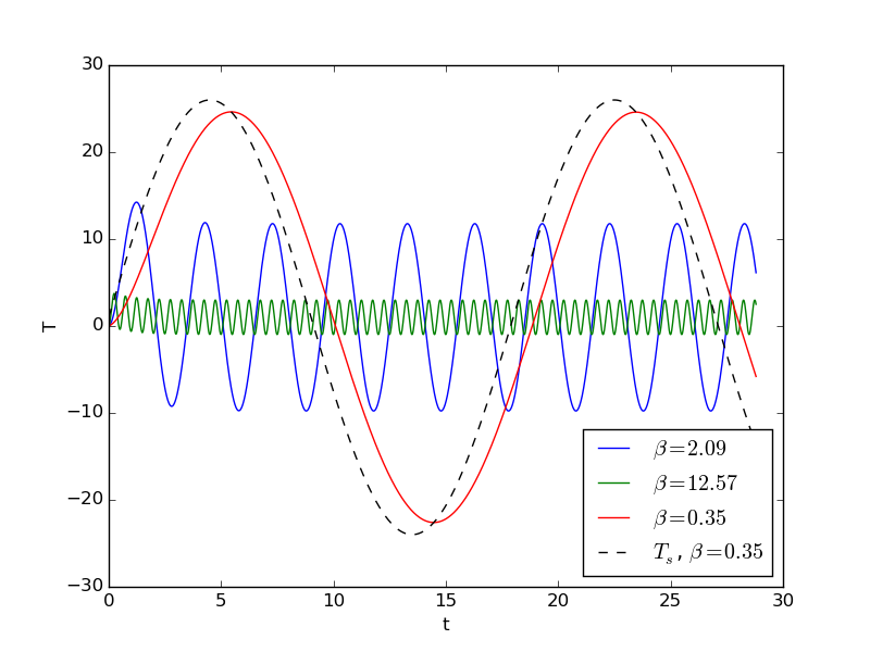
b) Consider the case where \(a\) is much larger than \(|T_m-T_0|\). What is an appropriate scaling of the temperature?
Problem 2.4: A nonlinear ODE for vertical motion with air resistance
The velocity \(v(t)\) of a body moving vertically through a fluid in the gravity field (with fluid drag, buoyancy, and added mass) is governed by the ODE
where \(t\) is time, \(m\) is the mass of the body, \(\mu\) is the body’s added mass, \(C_D\) is a drag coefficient, \(\varrho\) is the density of the fluid, \(A\) is the cross-sectional area perpendicular to the motion, \(g\) is the acceleration of gravity, and \(V\) is the volume of the body. Scale this ODE.
Filename: vertical_motion_with_drag.
Exercise 2.5: Solve a decay ODE with discontinuous coefficient
Make software for the problem in the section Variable coefficients so that you can produce Figure Exponential decay with jump: scaled model (left) and unscaled model (right).
Hint. Follow the ideas for software in the section Scaling a generalized problem: use the decay_vc.py module as computational engine and modify the falling_body.py code.
Filename: decay_jump.
Exercise 2.6: Implement a scaled model for cooling
Use software for the unscaled problem (17) to compute the solution of the scaled problem (24). Let \(T_s\) be a function of time.
Hint. You may use the general software decay_vc.py for computing with the cooling model. See the section Scaling a generalized problem for more ideas.
Filename: cooling1.
Problem 2.7: Decay ODE with discontinuous coefficients
The goal of this exercise is to scale the problem \(u^{\prime}(t) = -a(t)u(t) + b(t)\), \(u(0)=I\), when
Here, \(Q,A,\epsilon >0\).
Filename: decay_varcoeff.
Exercise 2.8: Alternative scalings of a cooling model
Implement the scaled model (30) and produce a plot with curves corresponding to various values of \(\alpha\) and \(p\) to summarize how \(\bar u(\bar t)\) looks like.
Hint. A centered Crank-Nicolson-style scheme for (30) can use an old time value for the nonlinear coefficient:
Filename: growth.
Exercise 2.9: Projectile motion
We have the following mathematical model for the motion of a projectile in two dimensions:
Here, \(m\) is the mass of the projectile, \(\boldsymbol{x}=x\boldsymbol{i} + y\boldsymbol{j}\) is the position vector of the projectile, \(\boldsymbol{i}\) and \(\boldsymbol{j}\) are unit vectors along the \(x\) and \(y\) axes, respectively, \(\ddot\boldsymbol{x}\) and \(\dot\boldsymbol{x}\) is the second- and first-order time derivative of \(\boldsymbol{x}(t)\), \(C_D\) is a drag coefficient depending on the shape of the projectile (can be taken as 0.4 for a sphere), \(\varrho\) is the density of the air, \(A\) is the cross section area (can be taken as \(\pi R^2\) for a sphere of radius \(R\)), \(g\) is gravity, \(v_0\) is the initial velocity of the projectile in a direction that makes the angle \(\theta\) with the ground.
a) Neglect the air resistance term proportional to \(\dot\boldsymbol{x}\) and solve analytically for \(\boldsymbol{x}(t)\).
b) Make the model for projectile motion with air resistance non-dimensional. Use the maximum height from the simplification in a) as length scale.
c) Make the model dimensionless again, but this time by demanding that the scaled initial velocity is unity in \(x\) direction.
d) A soccer ball has radius 11 cm and mass 0.43 kg, the density of air is 1.2 \(\hbox{kg}\hbox{m}^{-3}\), a soft kick has velocity 30 km/h, while a hard kick may have 120 km/h. Estimate the dimensionless parameter in the scaled problem for a soft and a hard kick with \(\theta\) corresponding to 45 degrees. Solve the scaled differential equation for these values and plot the trajectory (\(y\) versus \(x\)) for the two cases.
Filename: projectile.
Problem 2.10: A predator-prey model
The evolution of animal populations with a predator and a prey (e.g., lynx and hares, or foxes and rabbits) can be described by the Lotka-Volterra ODE system
Here, \(H\) is the number of animals of the prey (say hares) and \(L\) is the corresponding measure of the predator population (say lynx). There are six parameters: \(a\), \(b\), \(c\), \(d\), \(H_0\), and \(L_0\).
The terms have the following meanings:
- \(aH\) is the exponential population growth of \(H\) due to births and deaths and is governed by the access to nutrition,
- \(-bHL\) is the loss of preys because they are eaten by predators,
- \(dHL\) is the increase of predators because they eat preys (but only a fraction of the eaten preys, \(bHL\), contribute to population growth of the predator and therefore \(d < b\)),
- \(-cL\) is the exponential decay in the predator population because of deaths (the increase is modeled by \(dHL\)).
Dimensionless independent and dependent variables are introduced as usual by
where \(t_c\), \(H_c\), and \(L_c\) are scales to be determined. Inserted in the ODE problem we arrive at
a) Consider first a simple, intuitive scaling of \(H\) and \(L\) based on initial conditions \(H_c=H_0\) and \(L_c=H_c\). This means that \(\bar H\) starts out at unity and \(\bar L\) starts out as the fraction \(L_0/H_0\). Find a time scale and identify dimensionless parameters in the scaled ODE problem.
b) Try a different scaling where the aim is to adjust the scales such that the ODEs become as simple as possible, i.e, have as few dimensionless parameters as possible. Compare with the scaling in a).
c) A more mathematical approach to determining suitable scales for \(H\) and \(L\) consists in finding the stationary points \((H,L)\) of the ODE system, where \(H^{\prime}=L^{\prime}=0\), and use such points as characteristic sizes of the dependent variables. Show that \(H^{\prime}=L^{\prime}=0\) implies \(H=L=0\) or \(L=a/b\) and \(H=c/d\). Use \(H_c=a/b\), \(L_c=c/d\), and find a time scale. Compare with the result in b).
Filename: predator_prey.
Problem 2.11: A model for competing species
Let \(N_1(t)\) and \(N_2(t)\) be the number of animals in two competing species. A generalized Lotka-Volterra model is based on a logistic growth of each specie and a predator-prey like interaction (cf. Problem 2.10: A predator-prey model):
where \(r_1\), \(r_2\), \(M_1\), \(M_2\), \(s_{12}\), and \(s_{21}\) are given constants. The initial conditions specify \(N_1\) and \(N_2\) at \(t=0\). Find suitable scales and derive a dimensionless ODE problem.
Filename: competing_species.
Problem 2.12: Find the period of sinusoidal signals
This exercise aims at investigating various fundamental concepts like period, wave length, and frequency in non-damped and damped sinusoidal signals.
a) Plot the function
for \(t\in [0, 8\pi/\omega]\). Choose \(\omega\) and \(A\).
b) The period \(P\) of \(u\) is the shortest distance between two peaks (where \(u=A\)). Show mathematically that
Frequently, \(P\) is also referred to as the wave length of \(u\).
c) Plot the damped signal \(u(t)=e^{-at}\sin (\omega t)\) over four periods of \(sin(\omega t)\). Choose \(\omega\), \(A\), and \(a\).
d) What is the period of \(u(t)=e^{-at}\sin (\omega t)\)? We define the period \(P\) as the shortest distance between two peaks of the signal.
Hint. Use that \(v = p\cos(\omega t) + q\sin (\omega t)\) can be rewritten as \(v = B\cos(\omega t - \phi)\) with \(B=\sqrt{p^2 + q^2}\) and \(\phi = \tan^{-1}(p/q)\). Use such a rewrite of \(u'\) to find the peaks of \(u\) and then the period.
Filename: sine_period.
Remarks
The frequency is the number of up and down cycles in one unit time. Since there is one cycle in a period \(P\), the frequency is \(f =1/P\), measured in Hz. The angular frequency \(\omega\) is then \(\omega = 2\pi/P = 2\pi f\).
Problem 2.13: Oscillating mass with sliding friction
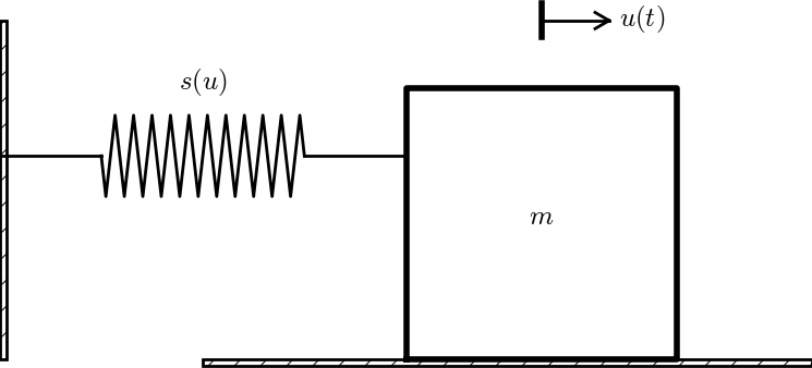
Body sliding on a surface
A mass attached to a spring is sliding on a surface and subject to a friction force, see Figure Body sliding on a surface. The spring represents a force \(-ku\boldsymbol{i}\), where \(k\) is the spring stiffness. The friction force is proportional to the normal force on the surface, \(-mg\boldsymbol{j}\), and given by \(-f(\dot u)\boldsymbol{i}\), where
Here, \(\mu \geq 0\) is a friction coefficient. With the signum function
we can simply write \(f(\dot u) = \mu mg\,\hbox{sign}(\dot u)\)
(the sign function is implemented by numpy.sign).
The ODE problem for this one-dimensional oscillatory motion reads
a) Scale the problem.
b) Implement the scaled model. Simulate for \(\alpha = 0, 0.05, 0.1\) and \(\beta =0\).
Filename: sliding_box.
Problem 2.14: Pendulum equations
The equation for a so-called simple pendulum with a mass \(m\) at the end is
where \(\theta(t)\) is the angle with the vertical, \(L\) is the length of the pendulum, and \(g\) is the acceleration of gravity.
A physical pendulum with moment of inertia \(I\) is governed by a similar equation,
Both equations have the initial conditions \(\theta(0)=\Theta\) and \(\theta'(0)=0\) (start at rest).
a) Use \(\theta\) as dimensionless unknown, find a proper time scale, and scale both differential equations.
b) Some may argue that \(\theta\) is not dimensionless since it is measured in radians. One may introduce a truly dimensionless angle \(\bar\theta \in [0,1]\). Set up the scaled ODE problem in this case.
c) Simulate the problem in b) for \(\Theta = 1,20,45,60\) measured in degrees.
Filename: pendulum.
Exercise 2.15: ODEs for a binary star
The equations for a binary star, or a planet and a moon, are
where \(\boldsymbol{x}_A\) is the position of object (star) A, and \(\boldsymbol{x}_B\) is the position object B. The corresponding masses are \(m_A\) and \(m_B\). The only force is the gravity force
where
and \(G\) is the gravitational constant: \(G=6.674\cdot 10^{-11}\hbox{ Nm}^2/\hbox{kg}^2\). A problem with these equations is that the parameters are very large (\(m_A\), \(m_B\), \(||\boldsymbol{r}||\)) or very small (\(G\)). The rotation time for binary stars can be very small and large as well.
a) Scale the equations.
b) Solve the scaled equations numerically for two cases:
- a planet around a star: \(\alpha = 10^{-3}\), \(\boldsymbol{x}_A(0)=(1,0)\), \(\dot\boldsymbol{x}_A(0)=(0,1)\), \(\boldsymbol{x}_B(0)=0\), \(\dot\boldsymbol{x}_B(0)=0\)
- two stars: \(\alpha = \frac{1}{2}\), \(\boldsymbol{x}_A(0)=(1,0)\), \(\dot\boldsymbol{x}_A(0)=(0,\frac{1}{2})\), \(\boldsymbol{x}_B(0)=0\), \(\dot\boldsymbol{x}_B(0)=(0,-\frac{1}{2})\)
An assumption here is that the orbits are co-planar such that they can be taken to lie in the \(xy\) plane.
Here is a movie of two rotating stars (point 2 above):
Filename: binary_star.
Problem 2.16: Duffing’s equation
Duffing’s equation is a vibration equation with linear and cubic spring terms:
Scale this problem.
Filename: Duffing_eq.
Problem 2.17: Vertical motion in a varying gravity field
A body (e.g., projectile or rocket) is launched vertically from the surface of the earth with velocity \(V\). The body’s distance (height) from the earth’s surface at time \(t\) is represented by the function \(h(t)\). Unless \(h\) is very much smaller than the earth’s radius \(R\), the motion takes place in a varying gravity field. The governing ODE problem for \(h(t)\) is then
where \(g\) is the acceleration of gravity at the earth’s surface.
The goal is to discuss three scalings of this problem. First we introduce
which gives the dimensionless ODE
and the dimensionless initial condition
The key dimensionless variable in this problem turns out to be
a) Assume we study the motion over long distances such that \(h\) may be of the same size as \(R\). In this case, \(h_c=R\) is a reasonable choice. Determine \(t_c\) from requiring the initial velocity to be unity. Set up the dimensionless ODE problem.
b) As a), but determine \(t_c\) by demanding both terms in the scaled ODE to have unit coefficients.
c) For small initial velocity \(V\), \(h\) will be small compared to \(R\). In the limit \(h/R\rightarrow 0\), the governing equation simplifies to the well-known motion in a constant gravity field: \(h''=-g\). Use this model to suggest a time and length scale, and derive a dimensionless ODE problem.
d) Give an interpretation of the dimensionless parameter \(\epsilon\).
e) Solve numerically for \(\bar h(\bar t)\) in each of the three scalings in a), b), and c), with \(\epsilon^2 =0.01, 0.1, 0.5, 1, 2\). When are the various scalings appropriate? (That is, when are \(\bar t\) and \(\bar h\) of size unity or at least not very small or big?)
Filename: varying_gravity.
Problem 2.18: A simplified Schroedinger equation
A simplified stationary Schroedinger’s equation for one electron, assuming radial symmetry, takes the form
where \(r\) is the radial coordinate, \(R\) is the wave function, \(\hbar\) is Planck’s constant, \(m\) is the mass of the electron, \(V=\) is the force potential, which is here taken as the Coulomb potential \(V(r) = {e^2}/(8\pi\epsilon_0 r)\) (where \(e\) is the charge of the electron and \(\epsilon_0\) is the permittivity of free space), and \(E\) is the eigenvalue, for the energy, to be determined along with \(R(r)\).
Show that the scaled version of (110) can be written
where \(\lambda\) is a dimensionless eigenvalue
The symbol \(\bar r\) is the scaled coordinate, and \(\bar R\) is a scaled version of \(R\) (the scaling factor drops out of the equation). The length scale, which arises naturally, is the Bohr radius.
Filename: Schroedinger.
Remarks
Introducing \(u=\bar r\bar R\) and renaming \(\bar r\) to \(x\), (111) can be recast in the simpler form
which is a simpler eigenvalue problem to solve numerically (the boundary conditions are \(u(0)=0\) and \(\lim_{x\rightarrow\infty}u(x)=0\)).