The diffusion equation

The diffusion equation in a one-dimensional homogeneous medium reads $$ \begin{equation} \frac{\partial u}{\partial t} = \dfc\frac{\partial^2 u}{\partial x^2}, \quad x\in (0,L),\ t\in (0,T], \tag{3.36} \end{equation} $$ where $ \dfc $ is the diffusion coefficient. The multi-dimensional generalization to a heterogeneous medium and a source term takes the form $$ \begin{equation} \frac{\partial u}{\partial t} = \nabla\cdot\left(\dfc \nabla u\right) + f, \quad x,y,z\in \Omega,\ t\in (0,T]\tp \tag{3.37} \end{equation} $$ We first look at scaling of the PDE itself, and thereafter we discuss some types of boundary conditions and how to scale the complete initial-boundary value problem.

Homogeneous 1D diffusion equation

Choosing the time scale

To make (3.36) dimensionless, we introduce, as usual, dimensionless dependent and independent variables: $$ \bar x = \frac{x}{x_c}, \quad \bar t = \frac{t}{t_c}, \quad \bar u =\frac{u}{u_c}\tp$$ Inserting the dimensionless quantities in the one-dimensional PDE (3.36) results in $$ \frac{\partial \bar u}{\partial \bar t} = \frac{t_c\dfc}{L^2} \frac{\partial^2 \bar u}{\partial \bar x^2}, \quad \bar x\in (0,1),\ \bar t\in (0,\bar T = T/t_c]\tp \tag{3.38} $$ Arguing, as for the wave equation, that the scaling should result in $$ \frac{\partial \bar u}{\partial \bar t}\hbox{ and } \frac{\partial^2 \bar u}{\partial \bar x^2}$$ of the same size (about unity), implies $ t_c\dfc/L^2=1 $ and therefore $ t_c = L^2/\dfc $.

Analytical insight

The best way to obtain the scales inherent in a problem is to obtain an exact analytic solution, as we have done in many of the ODE examples in this booklet. However, as a rule this is not possible. Still, often highly simplified analytic solutions can be found for parts of the problem, or for some closely related problem. Such solutions may provide crucial guidance to the nature of the complete solution and to the appropriate scaling of the full problem. We will employ such solutions now to learn about scales in diffusion problems.

One can show that $ u=Ae^{-pt}\sin (kx) $ is a solution of (3.36) if $ p=\dfc k^2 $, for any $ k $. This is the typical solution arising from separation of variables and reflects the dynamics of the space and time in the PDE. Exponential decay in time is a characteristic feature of diffusion processes, and the e-folding time can then be taken as a time scale. This means $ t_c = 1/p \sim k^{-2} $. Since $ k $ is related to the spatial wave length $ \lambda $ through $ k=2\pi/\lambda $, it means that $ t_c $ depends strongly on the wave length of the sine term $ \sin(kx) $. In particular, short waves (as found in noisy signals) with large $ k $ decay very rapidly. For the overall solution we are interested in how the longest meaningful wave decays and use that time scale for $ t_c $. The longest wave typically has half a wave length over the domain $ [0,L] $: $ u = Ae^{-pt}\sin(\pi x/L) $ ($ k=\pi/L $), provided $ u(0,t)=u(L,t)=0 $ (with $ u_x(L,t)=0 $, the longest wave is $ L/4 $, but we look at the case with the wave length $ L/2 $). Then $ t_c=L^2/\dfc \pi^{-2} $, but the factor $ \pi^{-2} $ is not important and we simply choose $ t_c=L^2/\dfc $, which equals the time scale we arrived at above. We may say that $ t_c $ is the time it takes for the diffusion to significantly change the solution in the entire domain.

Another fundamental solution of the diffusion equation is the diffusion of a Gaussian function: $ u(x,t)=K(4\pi\dfc t)^{-1/2}\exp{(-x^2/(4\dfc t))} $, for some constant $ K $ with the same dimension as $ u $. For the diffusion to be significant at a distance $ x=L $, we may demand the exponential factor to have a value of $ e^{-1}\approx 0.37 $, which implies $ t=L^2/(4\dfc) $, but the factor 4 is not of importance, so again, a relevant time scale is $ t_c=L^2/\dfc $.

Choosing other scales

The scale $ u_c $ is chosen according to the initial condition: $ u_c=\max_{x\in(0,L)}|I(x)| $. For a diffusion equation $ u_t=\dfc u_{xx} $ with $ u=0 $ at the boundaries $ x=0,L $, the solution is bounded by the initial condition $ I(x) $. Therefore, the listed choice of $ u_c $ implies that $ |u|\leq 1 $. (The solution $ u=Ae^{-pt}\sin (kx) $ is such an example if $ k=n\pi/L $ for integer $ n $ such that $ u=0 $ for $ x=0 $ and $ x=L $.)

The resulting dimensionless PDE becomes $$ \begin{equation} \frac{\partial \bar u}{\partial \bar t} = \frac{\partial^2 \bar u}{\partial \bar x^2}, \quad \bar x\in (0,1),\ \bar t\in (0,\bar T], \tag{3.39} \end{equation} $$ with initial condition $$ \bar u(\bar x, 0) = \bar I(\bar x) = \frac{I(x_c\bar x)}{\max_x |I(x)|}\tp$$ Notice that (3.39) is without physical parameters, but there may be parameters in $ I(x) $.

Generalized diffusion PDE

Turning the attention to (3.37), we introduce the dimensionless diffusion coefficient $$ \bar\dfc(\bar x,\bar y,\bar z) = \dfc_c^{-1}\dfc (x_c\bar x, y_c\bar y, z_c\bar z),$$ typically with $$ \dfc_c = \max_{x,y,z}\dfc(x,y,z)\tp$$ The length scales are $$ \bar x = \frac{x}{x_c},\quad \bar y = \frac{y}{y_c},\quad \bar z = \frac{z}{z_c}\tp $$ We scale $ f $ in a similar fashion: $$ \bar f(\bar x, \bar y, \bar z, \bar t) = f_c^{-1}f(\bar xx_c, \bar yy_c \bar zz_c, \bar tt_c),$$ with $$ f_c = \max_{x,y,z,t}|f(x,y,z,t)|\tp$$ Also assuming that $ x_c=y_c=z_c=L $, and $ u_c=\max_{x,y,z}(I(x,y,z) $, we end up with the scaled PDE $$ \begin{equation} \frac{\partial \bar u}{\partial \bar t} = \bar\nabla\cdot\left(\bar\dfc \bar\nabla \bar u\right) + \beta\bar f, \quad \bar x,\bar y,\bar z\in \bar \Omega,\ \bar t\in (0,\bar T]\tp \tag{3.40} \end{equation} $$ Here, $ \bar\nabla $ means differentiation with respect to dimensionless coordinates $ \bar x $, $ \bar y $, and $ \bar z $. The dimensionless parameter $ \beta $ takes the form $$ \beta = \frac{t_cf_c}{u_c} = \frac{L^2}{\dfc} \frac{\max_{x,y,z,t}|f(x,y,z,t)|}{\max_{x,y,z}|I(x,y,z)|}\tp$$ The scaled initial condition is $ \bar u = \bar I $ as in the 1D case.

An alternative choice of $ u_c $ is to make the coefficient $ t_cf_c/u_c $ in the source term unity. The scaled PDE now becomes $$ \begin{equation} \frac{\partial \bar u}{\partial \bar t} = \bar\nabla\cdot\left(\bar\dfc \bar\nabla \bar u\right) + f, \tag{3.41} \end{equation} $$ but the initial condition features the $ \beta $ parameter: $$ \bar u(\bar x, \bar y, \bar z, 0) = \frac{I}{t_cf_c} = \beta^{-1}\bar I(\bar x,\bar y,\bar z)\tp $$

The $ \beta $ parameter can be interpreted as the ratio of the source term and the terms with $ u $: $$ \beta = \frac{f_c}{u_c/t_c}\sim \frac{|f|}{|u_t|},\quad \beta = \frac{f_c}{u_c/t_c} = \frac{f_c}{L^2/t_c u_c/L^2}\sim \frac{|f_c|}{|\dfc\nabla^2 u|}\tp $$

We may check that $ \beta $ is really non-dimensional. From the PDE, $ f $ must have the same dimensions as $ \partial u/\partial t $, i.e., $ [\Theta\hbox{T}^{-1}] $. The dimension of $ \dfc $ is more intricate, but from the term $ \dfc u_{xx} $ we know that $ u_{xx} $ has dimensions $ [\Theta\hbox{L}^{-2}] $, and then $ \dfc $ must have dimension $ [\hbox{L}^2\hbox{T}^{-1}] $ to match the target $ [\Theta\hbox{T}^{-1}] $. In the expression for $ \beta $ we get $ [\hbox{L}^2\Theta\hbox{T}^{-1}(\hbox{L}^2\hbox{T}^{-1}\Theta)^{-1}] $, which equals 1 as it should.

Jump boundary condition

A classical one-dimensional heat conduction problem goes as follows. An insulated rod at some constant temperature $ U_0 $ is suddenly heated from one end ($ x=0 $), modeled as a constant Dirichlet condition $ u(0,t)=U_1\neq U_0 $ at that end. That is, the boundary temperature jumps from $ U_0 $ to $ U_1 $ at $ t=0 $. All the other surfaces of the rod are insulated such that a one-dimensional model is appropriate, but we must explicitly demand $ u_x(L,t)=0 $ to incorporate the insulation condition in the one-dimensional model at the end of the domain $ x=L $. Heat cannot escape, and since we supply heat at $ x=0 $, all of the material will eventually be warmed up to the temperature $ U_1 $: $ u\rightarrow U_1 $ as $ t\rightarrow\infty $.

The initial-boundary value problem reads $$ \begin{alignat}{2} \varrho c \frac{\partial u}{\partial t} &= k \frac{\partial^2 u}{\partial x^2}, \quad & x\in (0,L),\ t\in (0, T], \tag{3.42}\\ u(x,0) &= U_0, \quad & x\in [0,L], \tag{3.43}\\ u(0, t) & = U_1, \quad & t\in (0, T], \tag{3.44}\\ \frac{\partial}{\partial x} u(L, t) & = 0, \quad & t\in (0, T]. \tag{3.45} \end{alignat} $$ The PDE (3.42) arises from the energy equation in solids and involves three physical parameters: the density $ \varrho $, the specific heat capacity parameter $ c $,a nd the heat conduction coefficient (from Fourier's law). Dividing by $ \varrho c $ and introducing $ \dfc = k/(\varrho c) $ brings (3.42) on the standard form (3.36). We just use the $ \dfc $ parameter in the following.

The natural dimensionless temperature for this problem is $$ \bar u = \frac{u - U_0}{U_1 - U_0},$$ since this choice makes $ \bar u\in [0,1] $. The reason is that $ u $ is bounded by the initial and boundary conditions (in the absence of a source term in the PDE), and we have $ \bar u(\bar x,0)=0 $, $ \bar u(\bar x,\infty)=1 $, and $ \bar u(0,\bar t)=1 $.

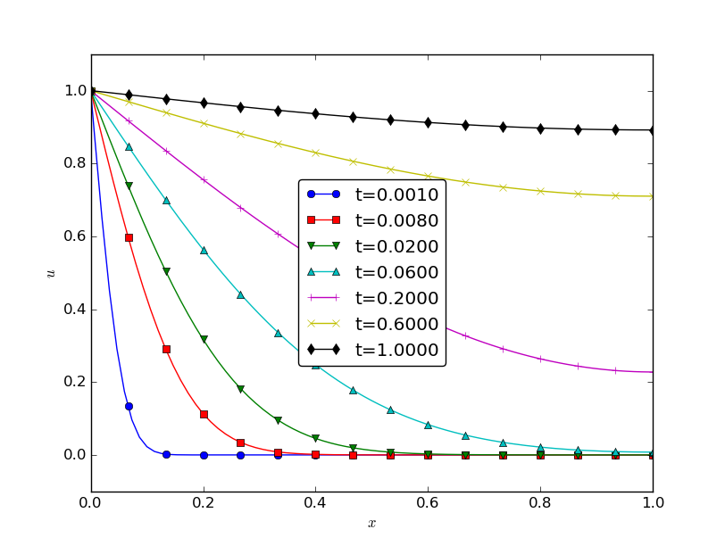
The choice of $ t_c $ is as in the previous cases. We arrive at the dimensionless initial-boundary value problem $$ \begin{alignat}{2} \frac{\partial \bar u}{\partial \bar t} &= \frac{\partial^2 \bar u}{\partial \bar x^2}, \quad & \bar x\in (0,1),\ \bar t\in (0, \bar T], \tag{3.46}\\ \bar u(\bar x,0) &= 0, \quad & \bar x\in [0,1], \tag{3.47}\\ \bar u(0, \bar t) & = 1, \quad & \bar t\in (0, \bar T], \tag{3.48}\\ \frac{\partial}{\partial \bar x} \bar u(1, \bar t) & = 0, \quad & \bar t\in (0, \bar T]. \tag{3.49} \end{alignat} $$ The striking feature is that there are no physical parameters left in this problem. One simulation can be carried out for $ \bar u(\bar x,\bar t) $, see Figure 15, and the temperature in a rod of any material and any constant initial and boundary temperature can be retrieved by $$ u(x,t) = U_0 + (U_1-U_0)\bar u(x/L, t\dfc/L^2)\tp$$

Figure 15: Scaled temperature in an isolated rod suddenly heated from the end.

Oscillating Dirichlet condition

Now we address a heat equation problem where the temperature is oscillating on the boundary $ x=0 $: $$ \begin{alignat}{2} \frac{\partial u}{\partial t} &= \dfc \frac{\partial^2 u}{\partial x^2}, \quad & x\in (0,L),\ t\in (0, T], \tag{3.50}\\ u(x,0) &= U_0, \quad & x\in [0,L], \tag{3.51}\\ u(0, t) & = U_0 + A\sin(\omega t), \quad & t\in (0, T], \tag{3.52}\\ \frac{\partial}{\partial x} u(L, t) & = 0, \quad & t\in (0, T]. \tag{3.53} \end{alignat} $$ One important physical application is temperature oscillations in the ground, either day and night variations at a short temporal and spatial scale, or seasonal variations in the Earth's crust. An important modeling assumption is (3.53), which means that the boundary $ x=L $ is placed sufficiently far from $ x=0 $ such that the solution is much damped and basically constant so $ u_x=0 $ is a reasonable condition.

Scaling issues

Since the boundary temperature is oscillating around the initial condition, we expect $ u\in [U_0-A,U_0+A] $. The dimensionless temperature is therefore taken as $$ \bar u = \frac{u-U_0}{A},$$ such that $ \bar u\in [-1,1] $.

What is an appropriate time scale? There will be two time scales involved, the oscillations $ \sin(\omega t) $ with period $ P=2\pi/\omega $ at the boundary and the "speed of diffusion", or more specifically the "speed of heat conduction" in the present context, where $ t_c=x_c^2/\dfc $ is the appropriate scale, $ x_c $ being the length scale. Choosing the right length scale is not obvious. As we shall see, the standard choice $ x_c=L $ is not a good candidate, but to understand why, we need to examine the solution, either through simulations or through a closed-form formula. We are so lucky in this relatively simple pedagogical problem that one can find an exact solution of a related problem.

Exact solution

As usual, investigating the exact solution of the model problem can illuminate the involved scales. For this particular initial-boundary value problem the exact solution as $ t\rightarrow\infty $ (such that the initial condition $ u(x,0)=U_0 $ is forgotten) and $ L\rightarrow\infty $ (such that (3.53) is certainly valid) can be shown to be $$ \begin{equation} u(x,t) = U_0 - Ae^{-bx}\sin (bx - \omega t),\quad b =\sqrt{\frac{\omega}{2\dfc}}\tp \tag{3.54} \end{equation} $$ This solution is of the form $ e^{-bx}g(x-ct) $, i.e., a damped wave that moves to the right with velocity $ c $ and a damped amplitude $ e^{-bx} $. This is perhaps more easily seen if we make a rewrite $$ u(x,t) = U_0 - Ae^{-bx}\sin\left(b(x - ct)\right),\quad c=\omega/b = \sqrt{2\dfc\omega},\ b =\sqrt{\frac{\omega}{2\dfc}}\tp$$

Time and length scales

The boundary oscillations lead to the time scale $ t_c=1/\omega $. The speed of the wave suggests another time scale: the time it takes to propagate through the domain, which is $ L/c $, and hence $ t_c = L/c = L/\sqrt{2\dfc\omega} $.

One can argue that $ L $ is not the appropriate length scale, because $ u $ is damped by $ e^{-bx} $. So, for $ x > 4/b $, $ u $ is close to zero. We may instead use $ 1/b $ as length scale, which is the e-folding distance of the damping factor, and base $ t_c $ on the time it takes a signal to propagate one length scale, $ t_c^{-1}=bc=\omega $. Similarly, the time scale based on the "speed of diffusion" changes to $ t_c^{-1}= b^2\dfc = \half\omega $ if we employ $ 1/b $ as length scale.

To summarize, we have three candidates for the time scale: $ t_c=L^2/\dfc $ (diffusion through the entire domain), $ t_c=2/\omega $ (diffusion through a distance $ 1/b $ where $ u $ is significantly different from zero), and $ t_c=1/\omega $ (wave movement over a distance $ 1/b $).

Let us look at the dimensionless exact solution to see if it can help with the choice of scales. We introduce the dimensionless parameters $$ \beta = bx_c = x_c\sqrt{\frac{\omega}{2\dfc}},\quad \gamma = \omega t_c\tp$$ The scaled solution becomes $$ \bar u(\bar x, \bar t; \beta,\gamma) = e^{-\beta\bar x}\sin(\gamma\bar t- \beta\bar x)\tp$$ The three choices of $ \gamma $, implied by the three choices of $ t_c $, are $$ \begin{equation} \gamma = \left\lbrace\begin{array}{ll} 1, & t_c=1/\omega,\\ 2, & t_c = 2/\omega,\\ 2\beta^2, & t_c = L^2/\dfc,\ x_c=L \end{array}\right. \tag{3.55} \end{equation} $$ The former two choices leave only $ \beta $ as parameter in $ \bar u $, and with $ x_c=1/b $ as length scale, $ \beta $ becomes unity, and there are no parameters in the dimensionless solution: $$ \begin{equation} \bar u(\bar x, \bar t) = e^{-\bar x}\sin(\bar t - \bar x)\tp \tag{3.56} \end{equation} $$ Therefore, $ x_c=1/b $ and $ t_c=1/\omega $ (or $ t_c=2/\omega $, but the factor 2 is of no importance) are the most appropriate scales.

To further argue why (3.56) demonstrates that these scales are preferred, think of $ \omega $ as large. Then the wave is damped over a short distance and there will be a thin boundary layer of temperature oscillations near $ x=0 $ and little changes in $ u $ in the rest of the domain. The scaling (3.56) resolves this problem by using $ 1/b \sim \omega^{-1/2} $ as length scale, because then the boundary layer thickness is independent of $ \omega $. The length of the domain can be chosen as, e.g., $ 4/b $ such that $ \bar u\approx 0 $ at the end $ x=L $. The length scale $ 1/b $ helps us to zoom in on the part of $ u $ where significant changes take place.

In the other limit, $ \omega $ small, $ b $ becomes small, and the wave is hardly damped in the domain $ [0,L] $ unless $ L $ is large enough. The imposed boundary condition on $ x=L $ in fact requires $ u $ to be approximately constant so its derivative vanishes, and this property can only be obtained if $ L $ is large enough to ensure that the wave becomes significantly damped. Therefore, the length scale is dictated by $ b $, not $ L $, and $ L $ should be adapted to $ b $, typically $ L\geq 4/b $ if $ e^{-4}\approx 0.018 $ is considered enough damping to consider $ \bar u\approx 0 $ for the boundary condition. This means that $ x\in [0,4/b] $ and then $ \bar x\in [0,4] $. Increasing the spatial domain to $ [0,6] $ implies a damping $ e^{-6}\approx 0.0025 $, if more accuracy is desired in the boundary condition.

The scaled problem

Based on the discussion of scales above, we arrive at the following scaled initial-boundary value problem: $$ \begin{alignat}{2} \frac{\partial \bar u}{\partial \bar t} &= \frac{1}{2}\frac{\partial^2\bar u}{\partial x^2}, \quad & \bar x\in (0,4),\ \bar t\in (0,\bar T], \tag{3.57}\\ \bar u(\bar x,0) &= 0, \quad &\bar x\in [0,1], \tag{3.58}\\ \bar u(0,\bar t) & = \sin(\bar t), \quad &\bar t\in (0,\bar T], \tag{3.59}\\ \frac{\partial}{\partial\bar x}\bar u(\bar L,\bar t) & = 0, \quad &\bar t\in (0,\bar T]. \tag{3.60} \end{alignat} $$ The coefficient in front of the second-derivative is $ \half $ because $$ \frac{t_c\dfc}{1/b^2} = \frac{b^2\dfc}{\omega} = \frac{1}{2}\tp$$ We may, of course, choose $ t_c=2/\omega $ and get rid of the $ \half $ factor, if desired, but then it turns up in (3.59) instead, as $ \sin (2\bar t) $.

The boundary condition at $ \bar x=\bar L $ is only an approximation and relies on sufficient damping of $ \bar u $ to consider it constant $ (\partial/\partial\bar x =0) $ in space. We could, therefore, assign the condition $ \bar u = 0 $ instead at $ \bar x=\bar L $.

Simulations

The file session.py contains a function solver_diffusion_FE for solving a diffusion equation in one dimension. This function can be used to solve the system (3.57)-(3.60), see diffusion_oscillatory_BC.

Diffusion wave.

Reaction-diffusion equations

Fisher's equation

Fisher's equation is essentially the logistic equation at each point for population dynamics (see the section Scaling a nonlinear ODE) combined with spatial movement through ordinary diffusion: $$ \begin{equation} \frac{\partial u}{\partial t} = \dfc\frac{\partial^2 u}{\partial x^2} + \varrho u(1-u/M) \tp \tag{3.61} \end{equation} $$ This PDE is also known as the KPP equation after Kolmogorov, Petrovsky, and Piskynov (who introduced the equation independently of Fisher).

Setting $$ \bar x = \frac{x}{x_c},\quad \ \bar t = \frac{t}{t_c}, \quad\bar u =\frac{u}{u_c},$$ results in $$ \frac{\partial \bar u}{\partial \bar t} = \frac{t_c\dfc}{x_c^2} \frac{\partial^2\bar u}{\partial\bar x^2} + t_c \varrho \bar u (1 - u_c\bar u/M)\tp $$

Balance of all terms

If all terms are equally important, the scales can be determined from demanding the coefficients to be unity. Reasoning as for the logistic ODE in the section Scaling a nonlinear ODE, we may choose $ t_c=1/\varrho $. Then the coefficient in the diffusion term dictates the length scale $ x_c = \sqrt{t_c\dfc} $. A natural scale for $ u $ is $ M $, since $ M $ is the upper limit of $ u $ in the model (cf. the logistic term). Summarizing, $$ u_c=M,\quad t_c = \frac{1}{\varrho},\quad x_c = \sqrt{\frac{\dfc}{\varrho}}, $$ and the scaled PDE becomes $$ \begin{equation} \frac{\partial \bar u}{\partial \bar t} = \frac{\partial^2 \bar u}{\partial\bar x^2} + \bar u (1 - \bar u)\tp \tag{3.62} \end{equation} $$ With this scaling, the length scale $ x_c=\sqrt{\dfc/\varrho} $ is not related to the domain size, so the scale is particularly relevant for infinite domains.

An open question is whether the time scale should be based on the diffusion process rather than the initial exponential growth in the logistic term. The diffusion time scale means $ t_c = x_c^2/\dfc $, but demanding the logistic term then to have a unit coefficient forces $ x_c^2\varrho /\dfc = 1 $, which implies $ x_c=\sqrt{\dfc/\varrho} $ and $ t_c=1/\varrho $. That is, equal balance of the three terms gives a unique choice of the time and length scale.

Fixed length scale

Assume now that we fix the length scale to be $ L $, either the domain size or some other naturally given length. With $ x_c=L $, $ t_c=\varrho^{-1} $, $ u_c=M $, we get $$ \begin{equation} \frac{\partial \bar u}{\partial \bar t} = \beta \frac{\partial^2 \bar u}{\partial\bar x^2} + \bar u (1 - \bar u), \tag{3.63} \end{equation} $$ where $ \beta $ is a dimensionless number $$ \beta = \frac{\dfc}{\varrho L^2} = \frac{\varrho^{-1}}{L^2/\dfc}\tp$$ The last equality demonstrates that $ \beta $ measures the ratio of the time scale for exponential growth in the beginning of the logistic process and the time scale of diffusion $ L^2/\dfc $ (i.e., the time it takes to transport a signal by diffusion through the domain). For small $ \beta $ we can neglect the diffusion and spatial movements, and the PDE is essentially a logistic ODE at each point, while for large $ \beta $, diffusion dominates, and $ t_c $ should in that case be based on the diffusion time scale $ L^2/\dfc $. This leads to the scaled PDE $$ \begin{equation} \frac{\partial \bar u}{\partial \bar t} = \frac{\partial^2 \bar u}{\partial\bar x^2} + \beta^{-1}\bar u (1 - \bar u), \tag{3.64} \end{equation} $$ showing that a large $ \beta $ encourages omission of the logistic term, because the point-wise growth takes place over long time intervals while diffusion is rapid. The effect of diffusion is then more prominent and it suffices to solve $ \bar u_{\bar t} = \bar u_{\bar x\bar x} $. The observant reader will in this latter case notice that $ u_c=M $ is an irrelevant scale for $ u $, since logistic growth with its limit is not of importance, so we implicitly assume that another scale $ u_c $ has been used, but that scale cancels anyway in the simplified PDE $ \bar u_{\bar t} = \bar u_{\bar x\bar x} $.

Nonlinear reaction-diffusion PDE

A general, nonlinear reaction-diffusion equation in 1D looks like $$ \begin{equation} \frac{\partial u}{\partial t} = \dfc\frac{\partial^2 u}{\partial x^2} + f(u) \tp \tag{3.65} \end{equation} $$ By scaling the nonlinear reaction term $ f(u) $ as $ f_c\bar f(u_c\bar u) $, where $ f_c $ is a characteristic size of $ f(u) $, typically the maximum value, one gets a non-dimensional PDE like $$ \frac{\partial\bar u}{\partial\bar t} = \frac{t_c\dfc}{x_c^2} \frac{\partial^2\bar u}{\partial\bar x^2} + \frac{t_cf_c}{u_c}\bar f(u_c\bar u)\tp $$ The characteristic size of $ u $ can often be derived from boundary or initial conditions, so we first assume that $ u_c $ is given. This fact uniquely determines the space and time scales by demanding that all three terms are equally important and of unit size: $$ t_c = \frac{u_c}{f_c},\quad x_c = \sqrt{\frac{\dfc u_c}{f_c}}\tp$$ The corresponding PDE reads $$ \begin{equation} \frac{\partial\bar u}{\partial\bar t} = \frac{\partial^2\bar u}{\partial\bar x^2} + \bar f(u_c\bar u)\tp \tag{3.66} \end{equation} $$

If $ x_c $ is based on some known length scale $ L $, balance of all three terms can be used to determine $ u_c $ and $ t_c $: $$ t_c = \frac{L^2}{\dfc},\quad u_c = \frac{L^2 f_c}{\dfc}\tp$$ This scaling only works if $ f $ is nonlinear, otherwise $ u_c $ cancels and there is no freedom to constrain this scale.

With given $ L $ and $ u_c $, there are two choices of $ t_c $ since it can be based on the diffusion or the reaction time scales. With the reaction scale, $ t_c = u_c/f_c $, one arrives a the PDE $$ \begin{equation} \frac{\partial\bar u}{\partial\bar t} = \beta\frac{\partial^2\bar u}{\partial\bar x^2} + \bar f(u_c\bar u), \tag{3.67} \end{equation} $$ where $$ \beta = \frac{\dfc u_c}{L^2 f_c} = \frac{u_c/f_c}{L^2/\dfc}$$ is a dimensionless number reflecting the ratio of the reaction time scale and the diffusion time scale. On the contrary, with the diffusion time scale, $ t_c=L^2/\dfc $, the scaled PDE becomes $$ \begin{equation} \frac{\partial\bar u}{\partial\bar t} = \frac{\partial^2\bar u}{\partial \bar x^2} + \beta^{-1}\bar f(u_c\bar u)\tp \tag{3.68} \end{equation} $$ The size of $ \beta $ in an application will determine which of the scalings that is most appropriate.