The convection-diffusion equation

Convection-diffusion without a force term

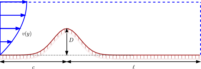
We now add a convection term $ \boldsymbol{v}\cdot\nabla u $ to the diffusion equation to obtain the well-known convection-diffusion equation: $$ \begin{equation} \frac{\partial u}{\partial t} + \v\cdot\nabla u = \dfc\nabla^2 u, \quad x,y, z\in \Omega,\ t\in (0, T]\tp \tag{3.69} \end{equation} $$ The velocity field $ \v $ is prescribed, and its characteristic size $ V $ is normally clear from the problem description. In the sketch below, we have some given flow over a bump, and $ u $ may be the concentration of some substance in the fluid. Here, $ V $ is typically $ \max_y v(y) $. The characteristic length $ L $ could be the entire domain, $ L=c+\ell $, or the height of the bump, $ L=D $. (The latter is the important length scale for the flow.)

Inserting $$ \bar x = \frac{x}{x_c},\ \bar y = \frac{y}{y_c},\ \bar z = \frac{z}{z_c}, \ \bar t = \frac{t}{t_c}, \ \bar\v = \frac{\v}{V}, \ \bar u =\frac{u}{u_c}$$ in (3.69) yields $$ \frac{u_c}{t_c} \frac{\partial \bar u}{\partial \bar t} + \frac{u_c V}{L}\bar\v\cdot\bar\nabla\bar u = \frac{\dfc u_c}{L^2}\bar\nabla^2\bar u, \quad \bar x,\bar y,\bar z\in \Omega,\ \bar t\in (0,\bar T]\tp $$ For $ u_c $ we simply introduce the symbol $ U $, which we may estimate from an initial condition. It is not critical here, since it vanishes from the scaled equation anyway, as long as there is no source term present. With some velocity measure $ V $ and length measure $ L $, it is tempting to just let $ t_c = L/V $. This is the characteristic time it takes to transport a signal by convection through the domain. The alternative is to use the diffusion length scale $ t_c=L^2/\dfc $. A common physical scenario in convection-diffusion problems is that the convection term $ \v\cdot\nabla u $ dominates over the diffusion term $ \dfc\nabla^2 u $. Therefore, the time scale for convection ($ L/V $) is most appropriate of the two. Only when the diffusion term is very much larger than the convection term (corresponding to very small Peclet numbers, see below) $ t_c=L^2/\dfc $ is the right time scale.

The non-dimensional form of the PDE with $ t_c=L/V $ becomes $$ \begin{equation} \frac{\partial \bar u}{\partial \bar t} + \bar\v\cdot\bar\nabla\bar u = \hbox{Pe}^{-1}\bar\nabla^2\bar u, \quad \bar x,\bar y,\bar z\in \Omega,\ \bar t\in (0,\bar T], \tag{3.70} \end{equation} $$ where Pe is the Peclet number, $$ \hbox{Pe} = \frac{LV}{\dfc}\tp$$ Estimating the size of the convection term $ \v\cdot\nabla u $ as $ VU/L $ and the diffusion term $ \dfc\nabla^2 u $ as $ \dfc U/L^2 $, we see that the Peclet number measures the ratio of the convection and the diffusion terms: $$ \hbox{Pe} = \frac{\hbox{convection}}{\hbox{diffusion}} = \frac{VU/L}{\dfc U/L^2}= \frac{LV}{\dfc}\tp $$

In case we use the diffusion time scale $ t_c=L^2/\dfc $, we get the non-dimensional PDE $$ \begin{equation} \frac{\partial \bar u}{\partial \bar t} + \hbox{Pe}\,\bar\v\cdot\bar\nabla\bar u = \bar\nabla^2\bar u, \quad \bar x,\bar y,\bar z\in \Omega,\ \bar t\in (0,\bar T]\tp \tag{3.71} \end{equation} $$

Discussion of scales and balance of terms in the PDE

We see that (3.70) and (3.71) are not equal, and they are based on two different time scales. For moderate Peclet numbers around 1, all terms have the same size in (3.70), i.e., a size around unity. For large Peclet numbers, (3.70) expresses a balance between the time derivative term and the convection term, both of size unity, and then there is a very small $ \hbox{Pe}^{-1}\bar\nabla^2\bar u $ term because Pe is large and $ \bar\nabla^2\bar u $ should be of size unity. That the convection term dominates over the diffusion term is consistent with the time scale $ t_c=L/V $ based on convection transport. In this case, we can neglect the diffusion term as Pe goes to infinity and work with a pure convection (or advection) equation $$ \frac{\partial \bar u}{\partial \bar t} + \bar\v\cdot\bar\nabla\bar u = 0\tp $$

For small Peclet numbers, $ \hbox{Pe}^{-1}\bar\nabla^2\bar u $ becomes very large and can only be balanced by two terms that are supposed to be unity of size. The time-derivative and/or the convection term must be much larger than unity, but that means we use suboptimal scales, since right scales imply that $ \partial\bar u/\partial\bar t $ and $ \bar v\cdot\bar\nabla\bar u $ are of order unity. Switching to a time scale based on diffusion as the dominating physical effect gives (3.71). For very small Peclet numbers this equation tells that the time-derivative balances the diffusion. The convection term $ \bar\v\cdot\bar\nabla\bar\u $ is around unity in size, but multiplied by a very small coefficient Pe, so this term is negligible in the PDE. An approximate PDE for small Peclet numbers is therefore $$ \frac{\partial \bar u}{\partial \bar t} = \bar\nabla^2\bar u\tp $$

Scaling can, with the above type of reasoning, be used to neglect terms from a differential equation under precise mathematical conditions.

Stationary PDE

Suppose the problem is stationary and that there is no need for any time scale. How is this type of convection-diffusion problem scaled? We get $$ \frac{VU}{L}\bar\v\cdot\bar\nabla\bar u = \frac{\dfc U}{L^2}\bar\nabla^2\bar u, $$ or $$ \begin{equation} \bar\v\cdot\bar\nabla\bar u = \hbox{Pe}^{-1}\bar\nabla^2\bar u\tp \tag{3.72} \end{equation} $$ This scaling only "works" for moderate Peclet numbers. For very small or very large Pe, either the convection term $ \bar\v\cdot\bar\nabla\bar u $ or the diffusion term $ \bar\nabla^2\bar u $ must deviate significantly from unity.

Consider the following 1D example to illustrate the point: $ \v = v\ii $, $ v>0 $ constant, a domain $ [0,L] $, with boundary conditions $ u(0)=0 $ and $ u(L)=U_L $. (The vector $ \ii $ is a unit vector in $ x $ direction.) The problem with dimensions is now $$ vu^{\prime} = \dfc u^{\prime\prime},\quad u(0)=0,\ u(L)=U_L\tp$$ Scaling results in $$ \frac{d\bar u}{d\bar x} = \hbox{Pe}^{-1}\frac{d^2\bar u}{d\bar x^2},\quad \bar x\in (0,1),\quad \bar u(0)=0,\ \bar u(1) = 1,$$ if we choose $ U=U_L $. The solution of the scaled problem is

\[ \bar u(\bar x) = \frac{1 - e^{\bar x{\small\hbox{Pe}}}}{1 - e^{\small\hbox{Pe}}}\tp\] Figure 16 indicates how $ \bar u $ depends on Pe: small Pe values give approximately a straight line while large Pe values lead to a boundary layer close to $ x=1 $, where the solution changes very rapidly.

Figure 16: Solution of scaled problem for 1D convection-diffusion.

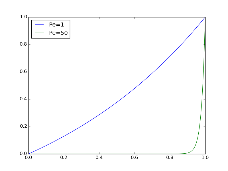
We realize that for large Pe, $$ \max_{\bar x}\frac{d\bar u}{d\bar x} \approx \hbox{Pe},\quad \max_{\bar x}\frac{d^2\bar u}{d\bar x^2} \approx \hbox{Pe}^{2},$$ which are consistent results with the PDE, since the double derivative term is multiplied by $ \hbox{Pe}^{-1} $. For small Pe, $$ \max_{\bar x}\frac{d\bar u}{d\bar x}\approx 1,\quad \max_{\bar x}\frac{d^2\bar u}{d\bar x^2} \approx 0,$$ which is also consistent with the PDE, since an almost vanishing second-order derivative is multiplied by a very large coefficient $ \hbox{Pe}^{-1} $. However, we have a problem with very large derivatives of $ \bar u $ when Pe is large.

To arrive at a proper scaling for large Peclet numbers, we need to remove the Pe coefficient from the differential equation. There are only two scales at our disposals: $ u_c $ and $ x_c $ for $ u $ and $ x $, respectively. The natural value for $ u_c $ is the boundary value $ U_L $ at $ x=L $. The scaling of $ Vu_x = \dfc u_{xx} $ then results in $$ \frac{d\bar u}{d\bar x} = \frac{\dfc}{Vx_c}\frac{d^2\bar u}{d\bar x^2}, \quad \bar x\in (0,\bar L),\quad \bar u(0)=0,\ \bar u(\bar L)=1,$$ where $ \bar L = L/x_c $. Choosing the coefficient $ \dfc/(Vx_c) $ to be unity results in the scale $ x_c=\dfc/V $, and $ \bar L $ becomes Pe. The final, scaled boundary-value problem is now $$ \frac{d\bar u}{d\bar x} = \frac{d^2\bar u}{d\bar x^2}, \quad \bar x \in (0, \hbox{Pe}), \quad \bar u(0)=0,\ \bar u(\hbox{Pe})=1,$$ with solution $$ \bar u(\bar x) = \frac{1 - e^{\bar x}}{1 - e^{\small\mbox{Pe}}}\tp$$ Figure 17 displays $ \bar u $ for some Peclet numbers, and we see that the shape of the graphs are the same with this scaling. For large Peclet numbers we realize that $ \bar u $ and its derivatives are around unity ($ 1-e^{\hbox{Pe}}\approx -e^{\small\hbox{Pe}} $), but for small Peclet numbers $ d\bar u/d\bar x \sim \hbox{Pe}^{-1} $.

Figure 17: Solution of scaled problem where the length scale depends on the Peclet number.

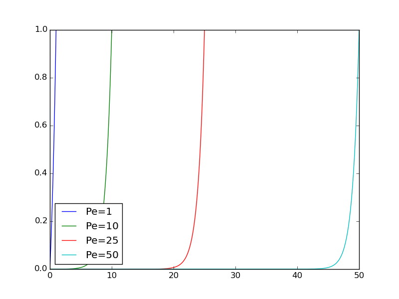
The conclusion is that for small Peclet numbers, $ x_c=L $ is an appropriate length scale. The scaled equation $ \hbox{Pe}\,\bar u' = \bar u'' $ indicates that $ \bar u''\approx 0 $, and the solution is close to a straight line. For large Pe values, $ x_c=\dfc/V $ is an appropriate length scale, and the scaled equation $ \bar u' = \bar u'' $ expresses that the terms $ \bar u' $ and $ \bar u'' $ are equal and of size around unity.

Convection-diffusion with a source term

Let us add a force term $ f(\x,t) $ to the convection-diffusion equation: $$ \begin{equation} \frac{\partial u}{\partial t} + \v\cdot\nabla u = \dfc\nabla^2 u + f\tp \tag{3.73} \end{equation} $$ The scaled version reads $$ \frac{\partial\bar u}{\partial\bar t} + \frac{t_cV}{L}\bar\v\cdot\bar\nabla \bar u = \frac{t_c\dfc}{L^2}\bar\nabla^2 \bar u + \frac{t_cf_c}{u_c}\bar f\tp $$ We can base $ t_c $ on convective transport: $ t_c = L/V $. Now, $ u_c $ could be chosen to make the coefficient in the source term unity: $ u_c = t_cf_c = Lf_c/V $. This leaves us with $$ \frac{\partial\bar u}{\partial\bar t} + \bar\v\cdot\bar \nabla\bar u = \hbox{Pe}^{-1}\bar \nabla^2 \bar u + \bar f\tp $$

In the diffusion limit, we base $ t_c $ on the diffusion time scale: $ t_c=L^2/\dfc $, and the coefficient of the source term set to unity determines $ u_c $ according to $$ \frac{L^2 f_c}{\dfc u_c} = 1\quad\Rightarrow\quad u_c = \frac{L^2 f_c}{\dfc}\tp$$ The corresponding PDE reads $$ \frac{\partial\bar u}{\partial\bar t} + \hbox{Pe}\,\bar\v\cdot\bar \nabla\bar u = \bar\nabla^2 \bar u + \bar f, $$ so for small Peclet numbers, which we have, the convective term can be neglected and we get a pure diffusion equation with a source term.

What if the problem is stationary? Then there is no time scale and we get $$ \frac{V u_c}{L}\bar\v\cdot\bar \nabla \bar u = \frac{u_c \dfc}{L^2}\bar\nabla^2 \bar u + f_c\bar f, $$ or $$ \bar\v\cdot\bar \nabla \bar u = \hbox{Pe}^{-1}\bar\nabla^2 \bar u + \frac{f_c L}{V u_c}\bar f\tp $$ Again, choosing $ u_c $ such that the source term coefficient is unity leads to $ u_c= f_c L/V $. Alternatively, $ u_c $ can be based on the initial condition, with similar results as found in the sections on the wave and diffusion PDEs.

Exercises

Problem 3.1: Stationary Couette flow

A fluid flows between two flat plates, with one plate at rest while the other moves with velocity $ U_0 $. This classical flow case is known as stationary Couette flow.

a) Directing the $ x $ axis in the flow direction and letting $ y $ be a coordinate perpendicular to the walls, one can assume that the velocity field simplifies to $ \u = u(y)\ii $. Show from the Navier-Stokes equations that the boundary-value problem for $ u(y) $ is $$ u^{\prime\prime}(u) = 0,\quad u(0)=0,\ u(H)=U_0\tp$$ We have here assumed at $ y=0 $ corresponds to the plate at rest and that $ y=H $ represents the plate that moves. There are no pressure gradients present in the flow.

b) Scale the problem in a) and show that the result has no physical parameters left in the model: $$ \frac{d^2\bar u}{d\bar y^2} = 0,\quad \bar u(0)=0,\ \bar u(1)=1\tp$$

c) We can compute $ \bar u(\bar y) $ from one numerical simulation (or a straightforward integration of the differential equation). Set up the formula that finds $ u(y; H, u_0) $ from $ \bar u(\bar y) $ for any values of $ H $ and $ U_0 $.

Filename: stationary_Couette.

Remarks

The problem for $ u $ is a classical two-point boundary-value problem in applied mathematics and arises in a number of applications, where Couette flow is just one example. Heat conduction is another example: $ u $ is temperature, and the heat conduction equation for an insulated rod reduces to $ u^{\prime\prime}=0 $ under stationary conditions and no heat source. Controlling the end $ x=0 $ at 0 degrees Celsius the other end $ x=L $ at $ U_0 $ degrees Celsius, gives the same boundary conditions as in the above flow problem. The scaled problem is of course the same whether we have flow of fluid or heat.

Exercise 3.2: Couette-Poiseuille flow

Viscous fluid flow between two infinite flat plates $ z=0 $ and $ z=H $ is governed by $$ \begin{align} \mu u''(z) &= -\beta \tag{3.74}\\ u(0) &= 0, \tag{3.75}\\ u(H) &= U_0\tp \tag{3.76} \end{align} $$ Here, $ u(z) $ is the fluid velocity in $ x $ direction (perpendicular to the $ z $ axis), $ \mu $ is the dynamic viscosity of the fluid, $ \beta $ is a positive constant pressure gradient, and $ U_0 $ is the constant velocity of the upper plate $ z=H $ in $ x $ direction. The model represents Couette flow for $ \beta=0 $ and Poiseuille flow for $ U_0=0 $.

a) Find the exact solution $ u(z) $. Point out how $ \beta $ and $ U_0 $ influence the magnitude of $ u $.

b) Scale the problem.

Filename: Couette_wpressure.

Exercise 3.3: Pulsatile pipeflow

The flow of a viscous fluid in a straight pipe with circular cross section with radius $ R $ is governed by $$ \begin{alignat}{2} \varrho\frac{\partial u}{\partial t} &= \frac{\mu}{r}\frac{\partial}{\partial r} \left(r\frac{\partial u}{\partial r}\right) - P(t), & r\in (0,R),\ t\in (0,T],\\ \frac{\partial u}{\partial r}(0,t) &= 0, & t\in (0,T],\\ u(R,t) &= 0, & t\in (0,T],\\ u(r,0) &= 0, & r\in [0,R]. \end{alignat} $$ The quantity $ u(r,t) $ is the fluid velocity, $ P(t) $ is a given pressure gradient, $ \varrho $ is the fluid density, and $ \mu $ is the dynamic viscosity.

Assume $ P(t) = A\cos\omega t $. Scale the problem and identify appropriate dimensionless numbers. Thereafter, assume $ P(t) $ is a more complicated function, but still period with period $ p $. Discuss how the scaling can be extended to this case.

Filename: pipeflow.

Exercise 3.4: The linear cable equation

A key PDE in neuroscience is the cable equation, here given in its simplest linear form: $$ \begin{equation} \tau\frac{\partial u}{\partial t} = \lambda^2\frac{\partial^2 u}{\partial x^2} -u\tp \tag{3.77} \end{equation} $$ The unknown $ u $ is the voltage (measured in volt) associated with an electric current along one-dimensional dendrites ("cables") in neural networks, while $ \tau $ and $ \lambda $ are given parameters.

Scale (3.77) in three ways: 1) let all terms in the scaled equation have unit coefficients, 2) use the domain size $ L $ as spatial scale and base the time scale on diffusion, 3) use the domain size $ L $ as spatial scale and base the time scale on reaction, i.e., the $ -u $ term.

Filename: cable_eq.

Exercise 3.5: Heat conduction with discontinuous initial condition

Two pieces of metal at different temperature are brought in contact at $ t=0 $. The following initial-boundary value problem governs the temperature evolution in the two pieces: $$ \begin{alignat}{2} \frac{\partial u}{\partial t} &= \dfc\nabla^2 u,\ & \x\in\Omega,\ t\in (0,T],\\ u(\x,0)&=I(x), & \x\in \Omega, \tag{3.78}\\ -\dfc\frac{\partial u}{\partial n} &= h(u-u_S), & x\in\partial\Omega,\ t\in (0,T]. \tag{3.79} \end{alignat} $$ Here, $ u(\x,t) $ is the temperature, $ \dfc $ the effective heat diffusion coefficient (assuming both pieces are homogeneous and of the same type of metal), and $ u_S $ is the surrounding temperature. The domain $ \Omega $ consists of the two pieces $ \Omega_1 $ and $ \Omega_2 $: $ \Omega = \Omega_1\cup\Omega_2 $. The initial condition can be specified as $$ I(x) = \left\lbrace\begin{array}{ll} U_1, & \x\in\Omega_1,\\ U_2, & \x\in\Omega_2, \end{array}\right. $$ where $ U_1 $ and $ U_2 $ are the constant initial temperatures in each piece.

Thinking of two identical pieces $ \Omega_1 $ and $ \Omega_2 $ with shapes as bricks, it is tempting to develop a one-dimensional model, especially if the pieces are somewhat slender. We then expect the main temperature variations to take place in the $ x $ direction, where the $ x $ axis is perpendicular to the contact surface between the pieces. A simplified PDE problem, neglecting variations in the $ y $ and $ z $ directions, takes the form $$ \begin{alignat}{2} \frac{\partial v}{\partial t} &= \dfc \frac{\partial^2 v}{\partial x^2} -\frac{hP}{A}(v(x,t) -u_S),\ & x\in (0,L),\ t\in (0,T], \tag{3.80}\\ v(x,0)&=I(x), & x\in (0,L),\\ \dfc\frac{\partial v}{\partial x} &= h(v(x,t)-u_S), & x=0,\ t\in (0,T], \tag{3.81}\\ -\dfc\frac{\partial v}{\partial x} &= h(v(x,t)-u_S), & x=L,\ t\in (0,T], \tag{3.82} \end{alignat} $$ with $$ I(x) = \left\lbrace\begin{array}{ll} U_1, & x\in [0,L/2),\\ U_2, & x\in [L/2, L]\tp \end{array}\right. $$ The parameter $ P $ is the perimeter of the cross section and $ A $ is the area of the cross section. Scale this problem.

Filename: metal_pieces.

Remarks

We can derive (3.80)-(3.82) from (3.78)-(3.79). The idea is to integrate the governing PDE (3.80) in the two directions where we expect negligible variations, use the Gauss divergence theorem in these directions, and apply the cooling boundary condition. Let $ A $ be the cross section of the bricks. Integrating over $ A $ gives $$ \begin{align*} \int\limits_A \frac{\partial u}{\partial t}dydz &= \int\limits_A \dfc\left( \frac{\partial^2 u}{\partial x^2} + \frac{\partial^2 u}{\partial y^2} + \frac{\partial^2 u}{\partial z^2} \right)dydz \\ &=\int\limits_A \dfc \frac{\partial^2 u}{\partial x^2} dydz + \int\limits_A \dfc\left( \frac{\partial^2 u}{\partial y^2} + \frac{\partial^2 u}{\partial z^2} \right)dydz \\ & = \int\limits_A \dfc \frac{\partial^2 u}{\partial x^2} dydz + \dfc\int\limits_{\partial A}\frac{\partial u}{\partial n}ds\\ & = \int\limits_A \dfc \frac{\partial^2 u}{\partial x^2} dydz -h(v(x,t) -u_S)P\tp \end{align*} $$ The parameter $ P $ is the perimeter of the cross section $ A $. The function $ v(x,t) $ means $ u(\x,t) $ evaluated at the boundary $ \partial A $. Assuming $ u $ to vary little across the cross section $ A $, we can approximate the integrals by $ u $ evaluated at $ \partial A $ as $ v $: $$ \int\limits_A \frac{\partial u}{\partial t}dydz\approx A \frac{\partial}{\partial t} v(x,t), \quad \int\limits_A \dfc \frac{\partial^2 u}{\partial x^2} dydz \approx A \dfc \frac{\partial^2 v}{\partial x^2}, $$ where $ A $ now is the cross-section area. The result is the 1D initial-boundary value problem (3.80)-(3.82).

Problem 3.6: Scaling a welding problem

Welding equipment makes a very localized heat source that moves in time. We shall investigate the heating due to welding and choose, for maximum simplicity, a one-dimensional heat equation with a fixed temperature at the ends (a 2D or 3D model with cooling conditions at the boundaries would be of greater physical significance, but now the scaling is in focus). The effect of melting is not included in the heat equation. Our goal is to investigate alternative scalings through numerical experimentation.

The governing PDE problem reads $$ \begin{alignat*}{2} \varrho c\frac{\partial u}{\partial t} &= k\frac{\partial^2 u}{\partial x^2} + f, & x\in (0,L),\ t\in (0,T),\\ u(x,0) &= U_s, & x\in [0,L],\\ u(0,t) = u(L,t) &= U_s, & t\in (0,T]. \end{alignat*} $$ Here, $ u $ is the temperature, $ \varrho $ the density of the material, $ c $ a heat capacity, $ k $ the heat conduction coefficient, $ f $ is the heat source from the welding equipment, and $ U_s $ is the initial constant (room) temperature in the material.

The boundary conditions at $ x=0,L $ are set for convenience – some sort of heat flux out of the boundary, modeled in terms of a cooling condition $ -ku_x = h(u-U_s) $, for a heat transfer coefficient $ h $, would yield a more physically relevant model. Also, only a full 3D geometry with such heat loss at the boundary is physically relevant, as neglecting a space dimension means insulated boundaries perpendicular to this direction. However, since the focus is on scaling, we prefer to work with the simplest possible model, which is one-dimensional, has Dirichlet boundary conditions, and neglects melting. The latter effect is very local and just stalls the temperature field locally – it does not affect the transport of heat away from the welding source in a significant way.

A possible model for the heat source is a moving Gaussian function: $$ f = A\exp{\left(-\frac{1}{2}\left(\frac{x-vt}{\sigma}\right)^2\right)},$$ where $ A $ is the strength, $ \sigma $ is a parameter governing how peak-shaped (or localized in space) the heat source is, and $ v $ is the velocity (in positive $ x $ direction) of the source.

a) Let $ x_c $, $ t_c $, $ u_c $, and $ f_c $ be scales, i.e., characteristic sizes, of $ x $, $ t $, $ u $, and $ f $, respectively. The natural choice of $ x_c $ and $ f_c $ is $ L $ and $ A $, since these make the scaled $ x $ and $ f $ in the interval $ [0,1] $. If each of the three terms in the PDE are equally important, we can find $ t_c $ and $ u_c $ by demanding that the coefficients in the scaled PDE are all equal to unity. Perform this scaling. Use scaled quantities in the arguments for the exponential function in $ f $ too and show that $$ \bar f= \exp{(-\frac{1}{2}\beta^2(\bar x -\gamma \bar t)^2)},$$ where $ \beta $ and $ \gamma $ are dimensionless numbers. Give an interpretation of $ \beta $ and $ \gamma $.

b) Argue that at least for large $ \gamma $ we should base the time scale on the movement of the heat source. Using $ L $ as length scale, show that this gives rise to the scaled PDE $$ \frac{\partial\bar u}{\partial\bar t} = \gamma^{-1}\frac{\partial^2\bar u}{\partial\bar x^2} + \bar f, $$ and $$ \bar f = \exp{(-\frac{1}{2}\beta^2(\bar x - \bar t)^2)}\tp$$ Discuss when the scalings in a) and b) are appropriate.

c) For fast movement of the welding equipment, i.e., when heat transfer is less important than the local heating by the equipment, the typical length scale of the local heating is the size of the source, reflected by the $ \sigma $ parameter. Modify the scaling in b) when $ \sigma $ is chosen as length scale.

d) A fourth kind of possible scaling is to say that for small $ \gamma $, the problem is quasi-stationary and the heat transfer balances the heat source. Determine $ u_c $ from this assumption. Use $ L $ as length scale and a time scale as in b), i.e., based on the movement of the welding equipment.

e) One aim with scaling is to get a solution that lies in the interval $ [-1,1] $. This is not always the case when $ u_c $ is based on a scale involving a source term, as we do in a)-c). However, from the scaled PDE we realize that if we replace $ \bar f $ with $ \delta\bar f $, where $ \delta $ is a dimensionless factor, this corresponds to replacing $ u_c $ by $ u_c/\delta $. So, if we observe that $ \bar u\sim1/\delta $ in simulations, we can just replace $ \bar f $ by $ \delta \bar f $ in the scaled PDE.

Use this trick and implement the four scaled models in a)-d). Reuse some software for the 1D diffusion equation. Make a function run(gamma, beta=10, delta=40, scaling=1, animate=False) that runs an implementation of the unscaled model with the given $ \gamma $, $ \beta $, and $ \delta $ parameters as well as an indicator scaling that is 'a', 'b', and so forth. The last argument can be used to turn screen animations on or off.

Perform experiments to find the proper value of $ \delta $ for each $ \gamma $ and for each scaling.

Equip the run function with visualization, both animation of $ \bar u $ and $ \bar f $, and plots with $ \bar u $ and $ \bar f $ for $ t=0.2 $ and $ t=0.5 $.

Hint.

Since the amplitudes of $ \bar u $ and $ \bar f $ differs by a factor $ \delta $, it is attractive to plot $ \bar f/\delta $ together with $ \bar u $.

f) Use the software in e) to investigate $ \gamma=0.2,1,5,40 $ for the four scalings. Discuss the results.

Filename: welding.