Study guide: Finite difference methods for vibration problems
Jul 14, 2016
A simple vibration problem
$$
u^{\prime\prime}(t) + \omega^2u = 0,\quad u(0)=I,\ u^{\prime}(0)=0,\ t\in (0,T]
$$
Exact solution:
$$
u(t) = I\cos (\omega t)
$$
\( u(t) \) oscillates with constant amplitude \( I \) and
(angular) frequency \( \omega \).
Period: \( P=2\pi/\omega \).
A centered finite difference scheme; step 1 and 2
- Strategy: follow the four steps of the finite difference method.
- Step 1: Introduce a time mesh, here uniform on \( [0,T] \): \( t_n=n\Delta t \)
- Step 2: Let the ODE be satisfied at each mesh point:
$$
u^{\prime\prime}(t_n) + \omega^2u(t_n) = 0,\quad n=1,\ldots,N_t
$$
A centered finite difference scheme; step 3
Step 3: Approximate derivative(s) by finite difference approximation(s). Very common (standard!) formula for \( u^{\prime\prime} \):
$$
u^{\prime\prime}(t_n) \approx \frac{u^{n+1}-2u^n + u^{n-1}}{\Delta t^2}
$$
Use this discrete initial condition together with the ODE at \( t=0 \) to eliminate \( u^{-1} \):
$$
\frac{u^{n+1}-2u^n + u^{n-1}}{\Delta t^2} = -\omega^2 u^n
$$
A centered finite difference scheme; step 4
Step 4: Formulate the computational algorithm. Assume \( u^{n-1} \) and \( u^n \) are known, solve for unknown \( u^{n+1} \):
$$
u^{n+1} = 2u^n - u^{n-1} - \Delta t^2\omega^2 u^n
$$
Nick names for this scheme: Stormer's method or Verlet integration.
Computing the first step
- The formula breaks down for \( u^1 \) because \( u^{-1} \) is unknown and outside the mesh!
- And: we have not used the initial condition \( u^{\prime}(0)=0 \).
Discretize \( u^{\prime}(0)=0 \) by a centered difference
$$
\frac{u^1-u^{-1}}{2\Delta t} = 0\quad\Rightarrow\quad u^{-1} = u^1
$$
Inserted in the scheme for \( n=0 \) gives
$$
u^1 = u^0 - \half \Delta t^2 \omega^2 u^0
$$
The computational algorithm
- \( u^0=I \)
- compute \( u^1 \)
- for \( n=1,2,\ldots,N_t-1 \):
- compute \( u^{n+1} \)
More precisly expressed in Python:
t = linspace(0, T, Nt+1)  # mesh points in time
dt = t[1] - t[0]          # constant time step.
u = zeros(Nt+1)           # solution

u[0] = I
u[1] = u[0] - 0.5*dt**2*w**2*u[0]
for n in range(1, Nt):
    u[n+1] = 2*u[n] - u[n-1] - dt**2*w**2*u[n]
Note: w is consistently used for \( \omega \) in my code.
Operator notation; ODE
With \( [D_tD_t u]^n \) as the finite difference approximation to \( u^{\prime\prime}(t_n) \) we can write
$$
[D_tD_t u + \omega^2 u = 0]^n
$$
\( [D_tD_t u]^n \) means applying a central difference with step \( \Delta t/2 \) twice:
$$ [D_t(D_t u)]^n = \frac{[D_t u]^{n+\half} - [D_t u]^{n-\half}}{\Delta t}$$
which is written out as
$$
\frac{1}{\Delta t}\left(\frac{u^{n+1}-u^n}{\Delta t} - \frac{u^{n}-u^{n-1}}{\Delta t}\right) = \frac{u^{n+1}-2u^n + u^{n-1}}{\Delta t^2}
\tp
$$
Operator notation; initial condition
$$
[u = I]^0,\quad [D_{2t} u = 0]^0
$$
where \( [D_{2t} u]^n \) is defined as
$$
[D_{2t} u]^n = \frac{u^{n+1} - u^{n-1}}{2\Delta t}
\tp
$$
Computing \( u^{\prime} \)
\( u \) is often displacement/position, \( u^{\prime} \) is velocity and can be computed by
$$
u^{\prime}(t_n) \approx \frac{u^{n+1}-u^{n-1}}{2\Delta t} = [D_{2t}u]^n
$$
Implementation
Core algorithm
import numpy as np
import matplotlib.pyplot as plt

def solver(I, w, dt, T):
    """
    Solve u'' + w**2*u = 0 for t in (0,T], u(0)=I and u'(0)=0,
    by a central finite difference method with time step dt.
    """
    dt = float(dt)
    Nt = int(round(T/dt))
    u = np.zeros(Nt+1)
    t = np.linspace(0, Nt*dt, Nt+1)

    u[0] = I
    u[1] = u[0] - 0.5*dt**2*w**2*u[0]
    for n in range(1, Nt):
        u[n+1] = 2*u[n] - u[n-1] - dt**2*w**2*u[n]
    return u, t

def solver_adjust_w(I, w, dt, T, adjust_w=True):
    """
    Solve u'' + w**2*u = 0 for t in (0,T], u(0)=I and u'(0)=0,
    by a central finite difference method with time step dt.
    """
    dt = float(dt)
    Nt = int(round(T/dt))
    u = np.zeros(Nt+1)
    t = np.linspace(0, Nt*dt, Nt+1)
    w_adj = w*(1 - w**2*dt**2/24.) if adjust_w else w

    u[0] = I
    u[1] = u[0] - 0.5*dt**2*w_adj**2*u[0]
    for n in range(1, Nt):
        u[n+1] = 2*u[n] - u[n-1] - dt**2*w_adj**2*u[n]
    return u, t
Plotting
def u_exact(t, I, w):
    return I*np.cos(w*t)

def visualize(u, t, I, w):
    plt.plot(t, u, 'r--o')
    t_fine = np.linspace(0, t[-1], 1001)  # very fine mesh for u_e
    u_e = u_exact(t_fine, I, w)
    plt.hold('on')
    plt.plot(t_fine, u_e, 'b-')
    plt.legend(['numerical', 'exact'], loc='upper left')
    plt.xlabel('t')
    plt.ylabel('u')
    dt = t[1] - t[0]
    plt.title('dt=%g' % dt)
    umin = 1.2*u.min();  umax = -umin
    plt.axis([t[0], t[-1], umin, umax])
    plt.savefig('tmp1.png');  plt.savefig('tmp1.pdf')
Main program
I = 1
w = 2*pi
dt = 0.05
num_periods = 5
P = 2*pi/w    #  one period
T = P*num_periods
u, t = solver(I, w, dt, T)
visualize(u, t, I, w, dt)
User interface: command line
import argparse
parser = argparse.ArgumentParser()
parser.add_argument('--I', type=float, default=1.0)
parser.add_argument('--w', type=float, default=2*pi)
parser.add_argument('--dt', type=float, default=0.05)
parser.add_argument('--num_periods', type=int, default=5)
a = parser.parse_args()
I, w, dt, num_periods = a.I, a.w, a.dt, a.num_periods
Running the program
Terminal> python vib_undamped.py --dt 0.05 --num_periods 40
Generates frames tmp_vib%04d.png in files. Can make movie:
Terminal> ffmpeg -r 12 -i tmp_vib%04d.png -c:v flv movie.flv
Can use avconv instead of ffmpeg.
| Format | Codec and filename |
|---|---|
| Flash | -c:v flv movie.flv |
| MP4 | -c:v libx264 movie.mp4 |
| Webm | -c:v libvpx movie.webm |
| Ogg | -c:v libtheora movie.ogg |
Verification
First steps for testing and debugging
- Testing very simple solutions: \( u=\hbox{const} \) or \( u=ct + d \) do not apply here (without a force term in the equation: \( u^{\prime\prime} + \omega^2u = f \)).
- Hand calculations: calculate \( u^1 \) and \( u^2 \) and compare with program.
Checking convergence rates
The next function estimates convergence rates, i.e., it
- performs \( m \) simulations with halved time steps: \( 2^{-k}\Delta t \), \( k=0,\ldots,m-1 \),
- computes the \( L_2 \) norm of the error, \( E = \sqrt{\Delta t_i\sum_{n=0}^{N_t-1}(u^n-\uex(t_n))^2} \) in each case,
- estimates the rates \( r_i \) from two consecutive experiments \( (\Delta t_{i-1}, E_{i-1}) \) and \( (\Delta t_{i}, E_{i}) \), assuming \( E_i=C\Delta t_i^{r_i} \) and \( E_{i-1}=C\Delta t_{i-1}^{r_i} \):
Implementational details
def convergence_rates(m, solver_function, num_periods=8):
    """
    Return m-1 empirical estimates of the convergence rate
    based on m simulations, where the time step is halved
    for each simulation.
    solver_function(I, w, dt, T) solves each problem, where T
    is based on simulation for num_periods periods.
    """
    from math import pi
    w = 0.35; I = 0.3       # just chosen values
    P = 2*pi/w              # period
    dt = P/30               # 30 time step per period 2*pi/w
    T = P*num_periods

    dt_values = []
    E_values = []
    for i in range(m):
        u, t = solver_function(I, w, dt, T)
        u_e = u_exact(t, I, w)
        E = np.sqrt(dt*np.sum((u_e-u)**2))
        dt_values.append(dt)
        E_values.append(E)
        dt = dt/2

    r = [np.log(E_values[i-1]/E_values[i])/
         np.log(dt_values[i-1]/dt_values[i])
         for i in range(1, m, 1)]
    return r, E_values, dt_values
Result: r contains values equal to 2.00 - as expected!
Unit test for the convergence rate
Use final r[-1] in a unit test:
def test_convergence_rates():
    r, E, dt = convergence_rates(
        m=5, solver_function=solver, num_periods=8)
    # Accept rate to 1 decimal place
    tol = 0.1
    assert abs(r[-1] - 2.0) < tol
    # Test that adjusted w obtains 4th order convergence
    r, E, dt = convergence_rates(
        m=5, solver_function=solver_adjust_w, num_periods=8)
    print 'adjust w rates:', r
    assert abs(r[-1] - 4.0) < tol

def plot_convergence_rates():
    r2, E2, dt2 = convergence_rates(
        m=5, solver_function=solver, num_periods=8)
    plt.loglog(dt2, E2)
    r4, E4, dt4 = convergence_rates(
        m=5, solver_function=solver_adjust_w, num_periods=8)
    plt.loglog(dt4, E4)
    plt.legend(['original scheme', r'adjusted $\omega$'],
               loc='upper left')
    plt.title('Convergence of finite difference methods')
    from plotslopes import slope_marker
    slope_marker((dt2[1], E2[1]), (2,1))
    slope_marker((dt4[1], E4[1]), (4,1))
    plt.savefig('tmp_convrate.png'); plt.savefig('tmp_convrate.pdf')
    plt.show()
Complete code in vib_undamped.py.
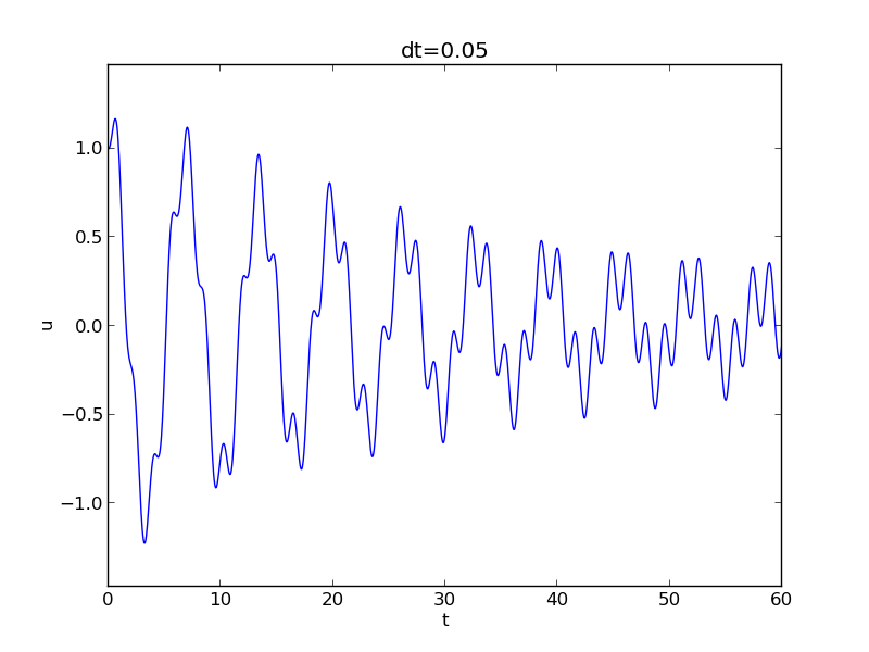
Long time simulations
Effect of the time step on long simulations
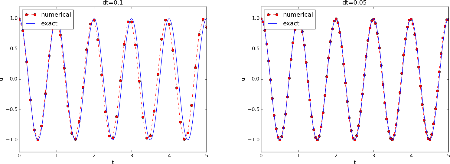
- The numerical solution seems to have right amplitude.
- There is an angular frequency error (reduced by reducing the time step).
- The total angular frequency error seems to grow with time.
Using a moving plot window
- In long time simulations we need a plot window that follows the solution.
- Method 1:
scitools.MovingPlotWindow. - Method 2:
scitools.avplotter(ASCII vertical plotter).
Example:
Terminal> python vib_undamped.py --dt 0.05 --num_periods 40
Movie of the moving plot window.
!splot
Long time simulations visualized with aid of Bokeh: coupled panning of multiple graphs
- Bokeh is a Python plotting library for fancy web graphics
- Example here: long time series with many coupled graphs that can move simultaneously
!splot
How does Bokeh plotting code look like?
def bokeh_plot(u, t, legends, I, w, t_range, filename):
    """
    Make plots for u vs t using the Bokeh library.
    u and t are lists (several experiments can be compared).
    legens contain legend strings for the various u,t pairs.
    """
    if not isinstance(u, (list,tuple)):
        u = [u]  # wrap in list
    if not isinstance(t, (list,tuple)):
        t = [t]  # wrap in list
    if not isinstance(legends, (list,tuple)):
        legends = [legends]  # wrap in list

    import bokeh.plotting as plt
    plt.output_file(filename, mode='cdn', title='Comparison')
    # Assume that all t arrays have the same range
    t_fine = np.linspace(0, t[0][-1], 1001)  # fine mesh for u_e
    tools = 'pan,wheel_zoom,box_zoom,reset,'\
            'save,box_select,lasso_select'
    u_range = [-1.2*I, 1.2*I]
    font_size = '8pt'
    p = []  # list of plot objects
    # Make the first figure
    p_ = plt.figure(
        width=300, plot_height=250, title=legends[0],
        x_axis_label='t', y_axis_label='u',
        x_range=t_range, y_range=u_range, tools=tools,
        title_text_font_size=font_size)
    p_.xaxis.axis_label_text_font_size=font_size
    p_.yaxis.axis_label_text_font_size=font_size
    p_.line(t[0], u[0], line_color='blue')
    # Add exact solution
    u_e = u_exact(t_fine, I, w)
    p_.line(t_fine, u_e, line_color='red', line_dash='4 4')
    p.append(p_)
    # Make the rest of the figures and attach their axes to
    # the first figure's axes
    for i in range(1, len(t)):
        p_ = plt.figure(
            width=300, plot_height=250, title=legends[i],
            x_axis_label='t', y_axis_label='u',
            x_range=p[0].x_range, y_range=p[0].y_range, tools=tools,
            title_text_font_size=font_size)
        p_.xaxis.axis_label_text_font_size = font_size
        p_.yaxis.axis_label_text_font_size = font_size
        p_.line(t[i], u[i], line_color='blue')
        p_.line(t_fine, u_e, line_color='red', line_dash='4 4')
        p.append(p_)

    # Arrange all plots in a grid with 3 plots per row
    grid = [[]]
    for i, p_ in enumerate(p):
        grid[-1].append(p_)
        if (i+1) % 3 == 0:
            # New row
            grid.append([])
    plot = plt.gridplot(grid, toolbar_location='left')
    plt.save(plot)
    plt.show(plot)
Analysis of the numerical scheme
Movie of the angular frequency error
\( u^{\prime\prime} + \omega^2 u = 0 \), \( u(0)=1 \), \( u^{\prime}(0)=0 \),
\( \omega=2\pi \), \( \uex(t)=\cos (2\pi t) \), \( \Delta t = 0.05 \) (20 intervals
per period)
We can derive an exact solution of the discrete equations
- We have a linear, homogeneous, difference equation for \( u^n \).
- Has solutions \( u^n \sim IA^n \), where \( A \) is unknown (number).
- Here: \( \uex(t) =I\cos(\omega t) \sim I\exp{(i\omega t)} = I(e^{i\omega\Delta t})^n \)
- Trick for simplifying the algebra: \( u^n = IA^n \), with \( A=\exp{(i\tilde\omega\Delta t)} \), then find \( \tilde\omega \)
- \( \tilde\omega \): unknown numerical frequency (easier to calculate than \( A \))
- \( \omega - \tilde\omega \) is the angular frequency error
- Use the real part as the physical relevant part of a complex expression
Calculations of an exact solution of the discrete equations
$$
u^n = IA^n = I\exp{(\tilde\omega \Delta t\, n)}=I\exp{(\tilde\omega t)} =
I\cos (\tilde\omega t) + iI\sin(\tilde \omega t)
\tp
$$
$$
\begin{align*}
[D_tD_t u]^n &= \frac{u^{n+1} - 2u^n + u^{n-1}}{\Delta t^2}\\
&= I\frac{A^{n+1} - 2A^n + A^{n-1}}{\Delta t^2}\\
&= I\frac{\exp{(i\tilde\omega(t+\Delta t))} - 2\exp{(i\tilde\omega t)} + \exp{(i\tilde\omega(t-\Delta t))}}{\Delta t^2}\\
&= I\exp{(i\tilde\omega t)}\frac{1}{\Delta t^2}\left(\exp{(i\tilde\omega(\Delta t))} + \exp{(i\tilde\omega(-\Delta t))} - 2\right)\\
&= I\exp{(i\tilde\omega t)}\frac{2}{\Delta t^2}\left(\cosh(i\tilde\omega\Delta t) -1 \right)\\
&= I\exp{(i\tilde\omega t)}\frac{2}{\Delta t^2}\left(\cos(\tilde\omega\Delta t) -1 \right)\\
&= -I\exp{(i\tilde\omega t)}\frac{4}{\Delta t^2}\sin^2(\frac{\tilde\omega\Delta t}{2})
\end{align*}
$$
Solving for the numerical frequency
The scheme with \( u^n=I\exp{(i\omega\tilde\Delta t\, n)} \) inserted gives
$$
-I\exp{(i\tilde\omega t)}\frac{4}{\Delta t^2}\sin^2(\frac{\tilde\omega\Delta t}{2})
+ \omega^2 I\exp{(i\tilde\omega t)} = 0
$$
which after dividing by \( I\exp{(i\tilde\omega t)} \) results in
$$
\frac{4}{\Delta t^2}\sin^2(\frac{\tilde\omega\Delta t}{2}) = \omega^2
$$
Solve for \( \tilde\omega \):
$$
\tilde\omega = \pm \frac{2}{\Delta t}\sin^{-1}\left(\frac{\omega\Delta t}{2}\right)
$$
- Frequency error because \( \tilde\omega \neq \omega \).
- Note: dimensionless number \( p=\omega\Delta t \) is the key parameter
(i.e., no of time intervals per period is important, not \( \Delta t \) itself) - But how good is the approximation \( \tilde\omega \) to \( \omega \)?
Polynomial approximation of the frequency error
Taylor series expansion for small \( \Delta t \) gives a formula that is easier to understand:
>>> from sympy import *
>>> dt, w = symbols('dt w')
>>> w_tilde = asin(w*dt/2).series(dt, 0, 4)*2/dt
>>> print w_tilde
(dt*w + dt**3*w**3/24 + O(dt**4))/dt  # note the final "/dt"
$$
\tilde\omega = \omega\left( 1 + \frac{1}{24}\omega^2\Delta t^2\right) + {\cal O}(\Delta t^3)
$$
The numerical frequency is too large (to fast oscillations).
Plot of the frequency error
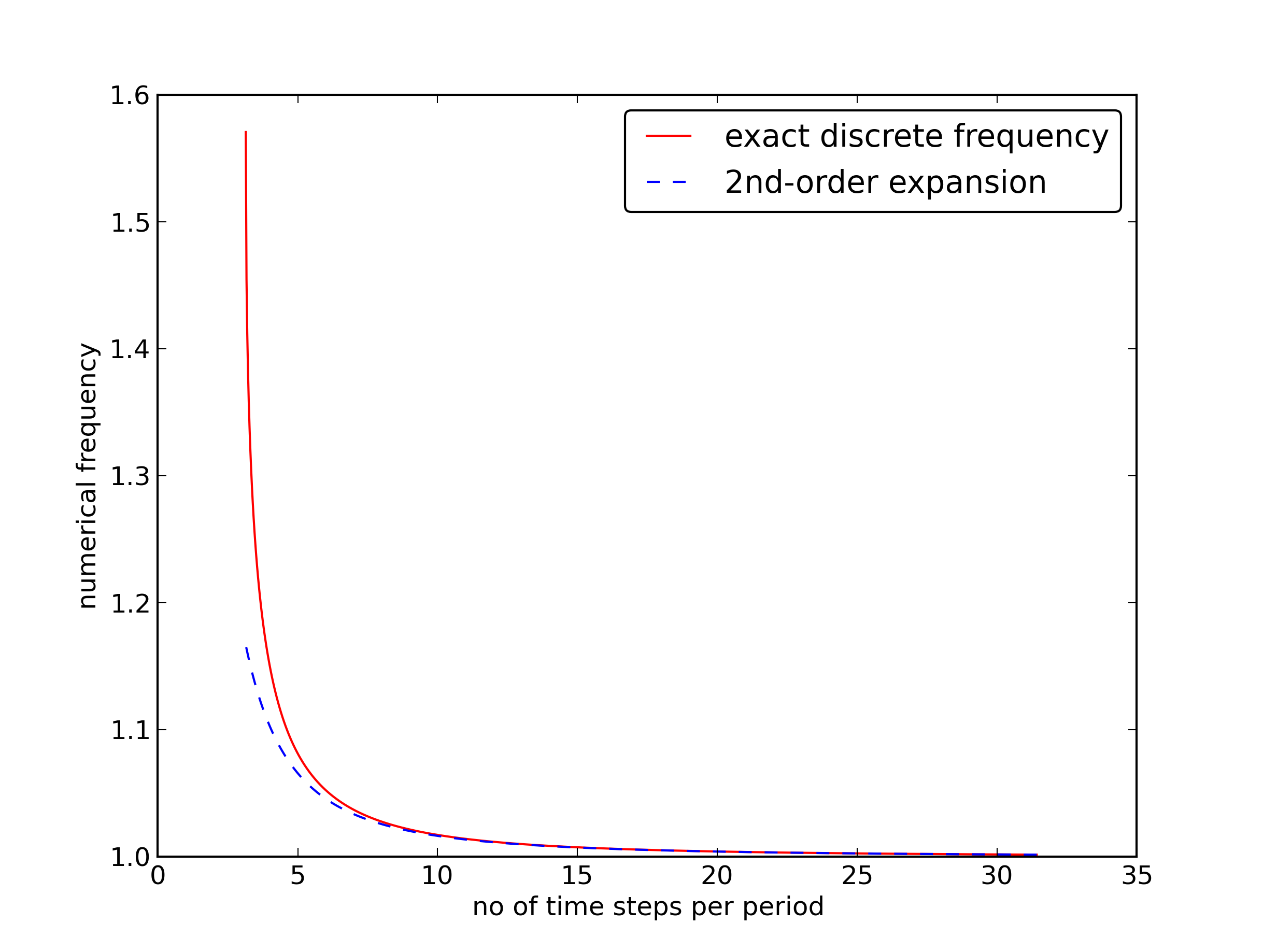
Recommendation: 25-30 points per period.
Exact discrete solution
$$
u^n = I\cos\left(\tilde\omega n\Delta t\right),\quad
\tilde\omega = \frac{2}{\Delta t}\sin^{-1}\left(\frac{\omega\Delta t}{2}\right)
$$
The error mesh function,
$$ e^n = \uex(t_n) - u^n =
I\cos\left(\omega n\Delta t\right)
- I\cos\left(\tilde\omega n\Delta t\right)
$$
is ideal for verification and further analysis!
$$
e^n = I\cos\left(\omega n\Delta t\right)
- I\cos\left(\tilde\omega n\Delta t\right)
= -2I\sin\left(t\half\left( \omega - \tilde\omega\right)\right)
\sin\left(t\half\left( \omega + \tilde\omega\right)\right)
$$
Convergence of the numerical scheme
Can easily show convergence:
$$ e^n\rightarrow 0 \hbox{ as }\Delta t\rightarrow 0,$$
because
$$
\lim_{\Delta t\rightarrow 0}
\tilde\omega = \lim_{\Delta t\rightarrow 0}
\frac{2}{\Delta t}\sin^{-1}\left(\frac{\omega\Delta t}{2}\right)
= \omega,
$$
by L'Hopital's rule or simply asking sympy:
or WolframAlpha:
>>> import sympy as sym
>>> dt, w = sym.symbols('x w')
>>> sym.limit((2/dt)*sym.asin(w*dt/2), dt, 0, dir='+')
w
Stability
Observations:
- Numerical solution has constant amplitude (desired!), but an angular frequency error
- Constant amplitude requires \( \sin^{-1}(\omega\Delta t/2) \) to be real-valued \( \Rightarrow |\omega\Delta t/2| \leq 1 \)
- \( \sin^{-1}(x) \) is complex if \( |x| > 1 \), and then \( \tilde\omega \) becomes complex
What is the consequence of complex \( \tilde\omega \)?
- Set \( \tilde\omega = \tilde\omega_r + i\tilde\omega_i \)
- Since \( \sin^{-1}(x) \) has a *negative* imaginary part for \( x>1 \), \( \exp{(i\omega\tilde t)}=\exp{(-\tilde\omega_i t)}\exp{(i\tilde\omega_r t)} \) leads to exponential growth \( e^{-\tilde\omega_it} \) when \( -\tilde\omega_i t > 0 \)
- This is instability because the qualitative behavior is wrong
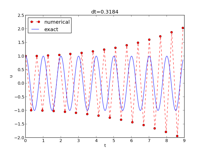
The stability criterion
Cannot tolerate growth and must therefore demand a stability criterion
$$
\frac{\omega\Delta t}{2} \leq 1\quad\Rightarrow\quad
\Delta t \leq \frac{2}{\omega}
$$
Try \( \Delta t = \frac{2}{\omega} + 9.01\cdot 10^{-5} \) (slightly too big!):
Summary of the analysis
We can draw three important conclusions:
- The key parameter in the formulas is \( p=\omega\Delta t \) (dimensionless)
- Period of oscillations: \( P=2\pi/\omega \)
- Number of time steps per period: \( N_P=P/\Delta t \)
- \( \Rightarrow\ p=\omega\Delta t = 2\pi/ N_P \sim 1/N_P \)
- The smallest possible \( N_P \) is 2 \( \Rightarrow \) $p\in (0,\pi]$
Alternative schemes based on 1st-order equations
Rewriting 2nd-order ODE as system of two 1st-order ODEs
The vast collection of ODE solvers (e.g., in Odespy) cannot be applied to
$$ u^{\prime\prime} + \omega^2 u = 0$$
unless we write this higher-order ODE as a system of 1st-order ODEs.
Introduce an auxiliary variable \( v=u^{\prime} \):
$$
\begin{align}
u^{\prime} &= v,
\tag{1}\\
v^{\prime} &= -\omega^2 u
\tag{2}
\tp
\end{align}
$$
Initial conditions: \( u(0)=I \) and \( v(0)=0 \).
The Forward Euler scheme
We apply the Forward Euler scheme to each component equation:
$$ [D_t^+ u = v]^n,$$
$$ [D_t^+ v = -\omega^2 u]^n,$$
or written out,
$$
\begin{align}
u^{n+1} &= u^n + \Delta t v^n,
\tag{3}\\
v^{n+1} &= v^n -\Delta t \omega^2 u^n
\tp
\tag{4}
\end{align}
$$
The Backward Euler scheme
We apply the Backward Euler scheme to each component equation:
$$ [D_t^- u = v]^{n+1},$$
$$ [D_t^- v = -\omega u]^{n+1} \tp $$
Written out:
$$
\begin{align}
u^{n+1} - \Delta t v^{n+1} = u^{n},
\tag{5}\\
v^{n+1} + \Delta t \omega^2 u^{n+1} = v^{n}
\tp
\tag{6}
\end{align}
$$
This is a coupled \( 2\times 2 \) system for the new values at \( t=t_{n+1} \)!
The Crank-Nicolson scheme
$$
[D_t u = \overline{v}^t]^{n+\half},$$
$$
[D_t v = -\omega \overline{u}^t]^{n+\half}$$
The result is also a coupled system:
$$
\begin{align}
u^{n+1} - \half\Delta t v^{n+1} &= u^{n} + \half\Delta t v^{n},
\tag{7}\\
v^{n+1} + \half\Delta t \omega^2 u^{n+1} &= v^{n}
- \half\Delta t \omega^2 u^{n}
\tp
\tag{8}
\end{align}
$$
Comparison of schemes via Odespy
Can use Odespy to compare many methods for first-order schemes:
import odespy
import numpy as np

def f(u, t, w=1):
    # v, u numbering for EulerCromer to work well
    v, u = u  # u is array of length 2 holding our [v, u]
    return [-w**2*u, v]

def run_solvers_and_plot(solvers, timesteps_per_period=20,
                         num_periods=1, I=1, w=2*np.pi):
    P = 2*np.pi/w  # duration of one period
    dt = P/timesteps_per_period
    Nt = num_periods*timesteps_per_period
    T = Nt*dt
    t_mesh = np.linspace(0, T, Nt+1)

    legends = []
    for solver in solvers:
        solver.set(f_kwargs={'w': w})
        solver.set_initial_condition([0, I])
        u, t = solver.solve(t_mesh)
Forward and Backward Euler and Crank-Nicolson
solvers = [
    odespy.ForwardEuler(f),
    # Implicit methods must use Newton solver to converge
    odespy.BackwardEuler(f, nonlinear_solver='Newton'),
    odespy.CrankNicolson(f, nonlinear_solver='Newton'),
    ]
Two plot types:
- \( u(t) \) vs \( t \)
- Parameterized curve \( (u(t), v(t)) \) in phase space
- Exact curve is an ellipse: \( (I\cos\omega t, -\omega I\sin\omega t) \), closed and periodic
Phase plane plot of the numerical solutions
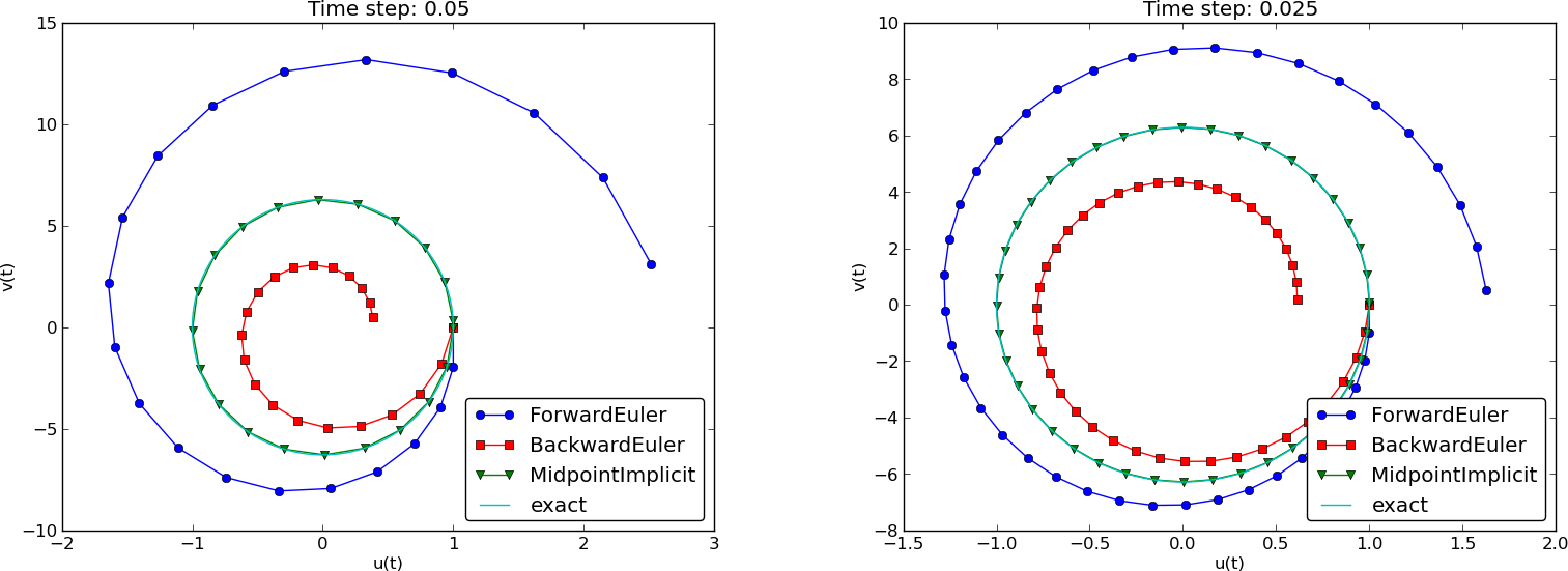
Note: CrankNicolson in Odespy leads to the name MidpointImplicit in plots.
Plain solution curves
Figure 1: Comparison of classical schemes.
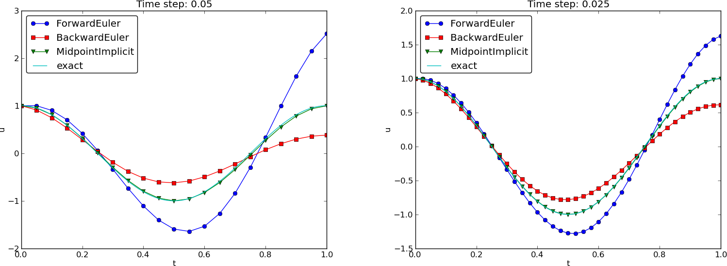
Observations from the figures
- Forward Euler has growing amplitude and outward \( (u,v) \) spiral - pumps energy into the system.
- Backward Euler is opposite: decreasing amplitude, inward sprial, extracts energy.
- Forward and Backward Euler are useless for vibrations.
- Crank-Nicolson (MidpointImplicit) looks much better.
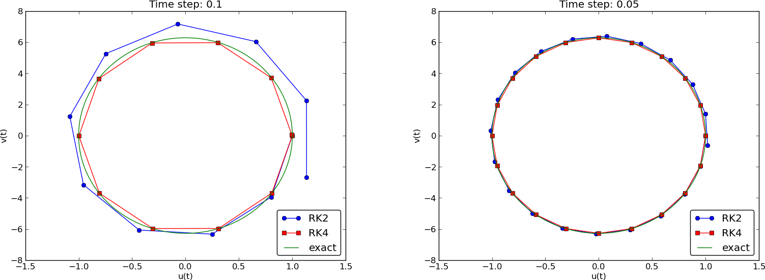
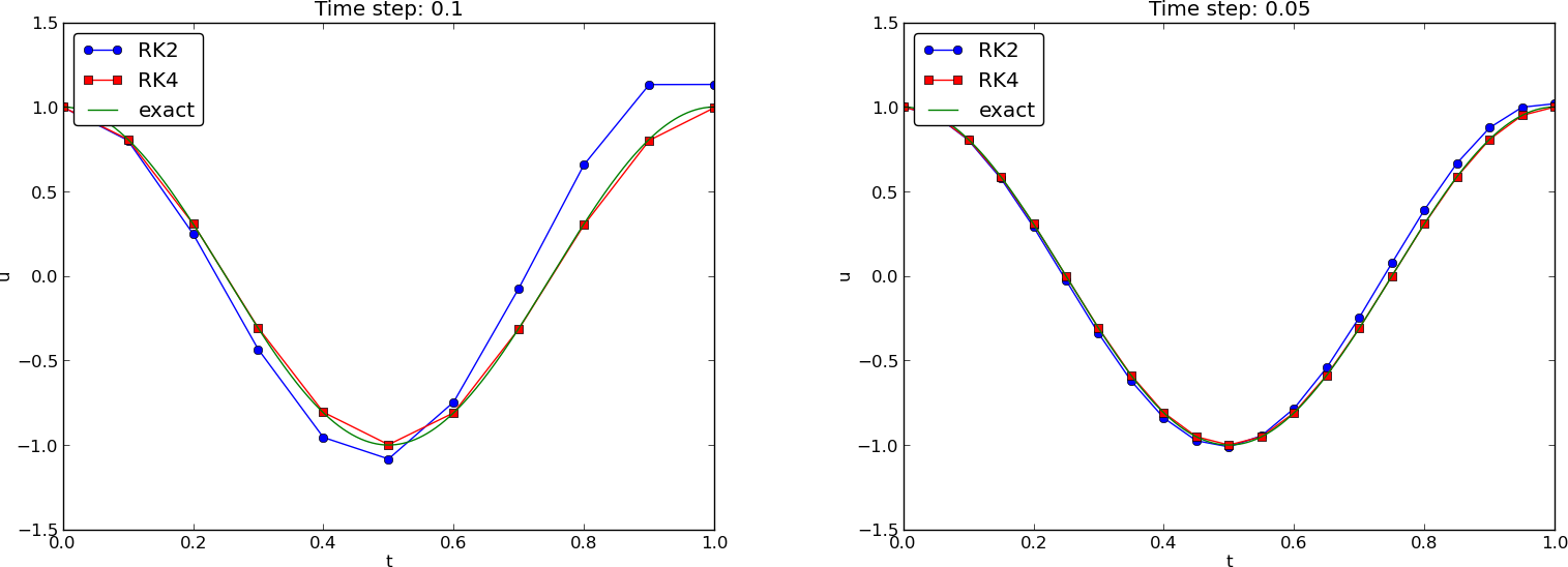
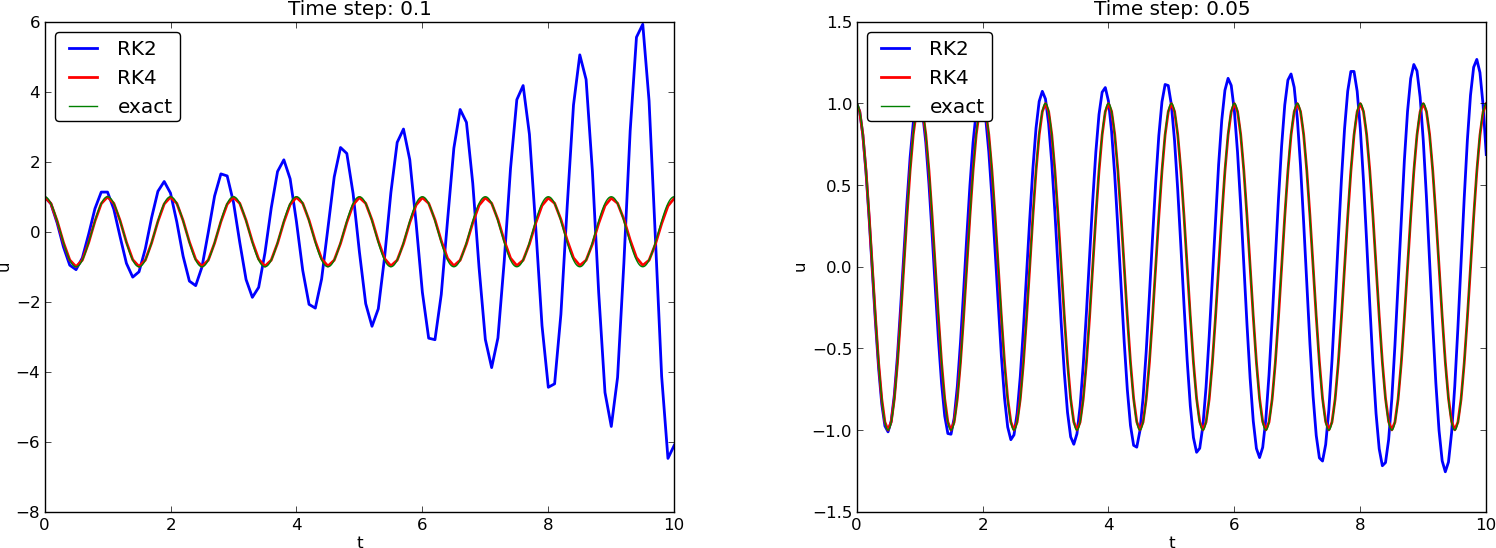
Runge-Kutta methods of order 2 and 4; short time series
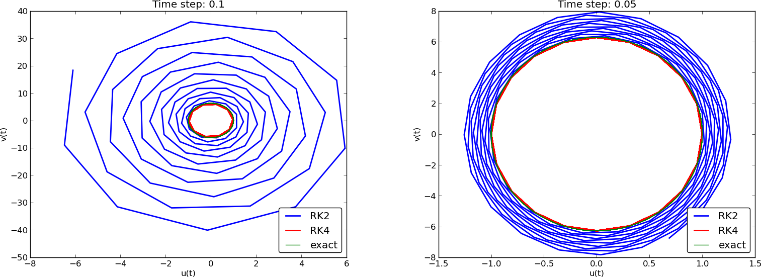
Runge-Kutta methods of order 2 and 4; longer time series
Crank-Nicolson; longer time series
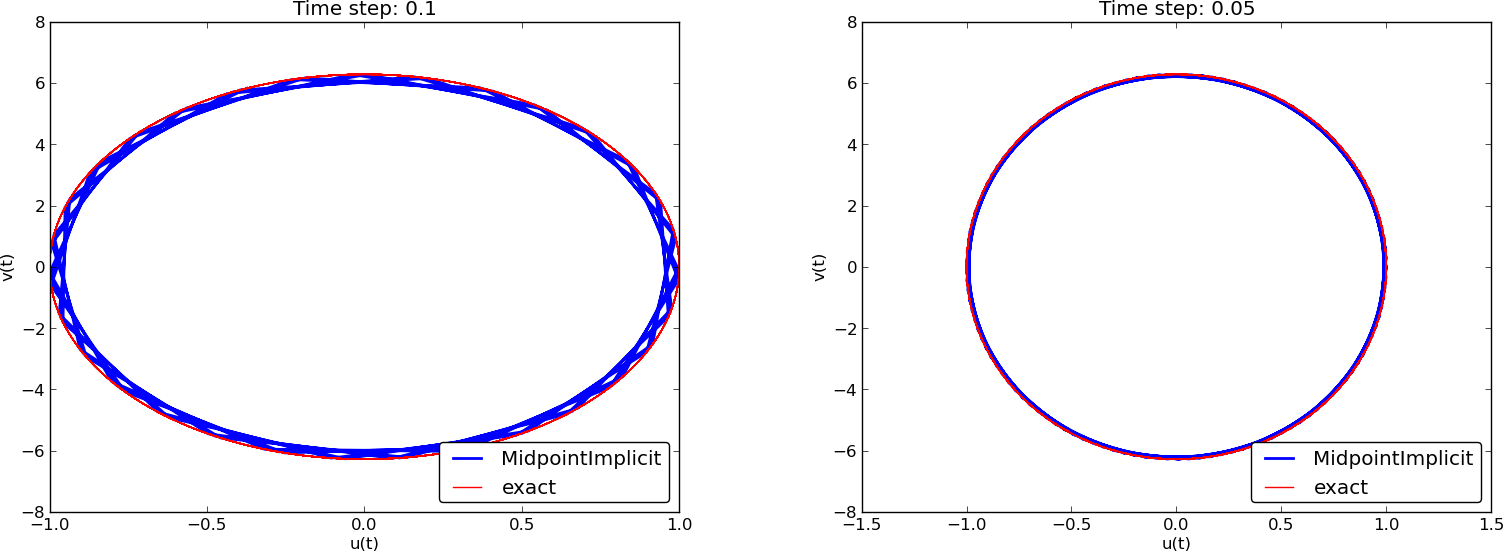
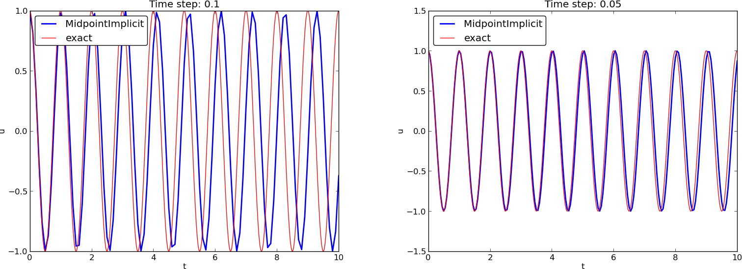
(MidpointImplicit means CrankNicolson in Odespy)
Observations of RK and CN methods
- 4th-order Runge-Kutta is very accurate, also for large \( \Delta t \).
- 2th-order Runge-Kutta is almost as bad as Forward and Backward Euler.
- Crank-Nicolson is accurate, but the amplitude is not as accurate as the difference scheme for \( u^{\prime\prime}+\omega^2u=0 \).
Energy conservation property
The model
$$ u^{\prime\prime} + \omega^2 u = 0,\quad u(0)=I,\ u^{\prime}(0)=V,$$
has the nice energy conservation property that
$$ E(t) = \half(u^{\prime})^2 + \half\omega^2u^2 = \hbox{const}\tp$$
This can be used to check solutions.
Derivation of the energy conservation property
Multiply \( u^{\prime\prime}+\omega^2u=0 \) by \( u^{\prime} \) and integrate:
$$ \int_0^T u^{\prime\prime}u^{\prime} dt + \int_0^T\omega^2 u u^{\prime} dt = 0\tp$$
Observing that
$$ u^{\prime\prime}u^{\prime} = \frac{d}{dt}\half(u^{\prime})^2,\quad uu^{\prime} = \frac{d}{dt} {\half}u^2,$$
we get
$$
\int_0^T (\frac{d}{dt}\half(u^{\prime})^2 + \frac{d}{dt} \half\omega^2u^2)dt = E(T) - E(0),
$$
where
$$
E(t) = \half(u^{\prime})^2 + \half\omega^2u^2
$$
Remark about \( E(t) \)
\( E(t) \) does not measure energy, energy per mass unit.
Starting with an ODE coming directly from Newton's 2nd law \( F=ma \) with a spring force \( F=-ku \) and \( ma=mu^{\prime\prime} \) (\( a \): acceleration, \( u \): displacement), we have
$$ mu^{\prime\prime} + ku = 0$$
Integrating this equation gives a physical energy balance:
$$
E(t) = \underbrace{{\half}mv^2}_{\hbox{kinetic energy} }
+ \underbrace{{\half}ku^2}_{\hbox{potential energy}} = E(0),\quad v=u^{\prime}
$$
Note: the balance is not valid if we add other terms to the ODE.
The Euler-Cromer method; idea
2x2 system for \( u^{\prime\prime}+\omega^2u=0 \):
$$
\begin{align*}
v^{\prime} &= -\omega^2u\\
u^{\prime} &= v
\end{align*}
$$
Forward-backward discretization:
- Update \( v \) with Forward Euler
- Update \( u \) with Backward Euler, using latest \( v \)
$$
\begin{align}
[D_t^+v &= -\omega^2u]^n
\tag{9}\\
[D_t^-u &= v]^{n+1}
\tag{10}
\end{align}
$$
The Euler-Cromer method; complete formulas
Written out:
$$
\begin{align}
u^0 &= I,
\tag{11}\\
v^0 &= 0,
\tag{12}\\
v^{n+1} &= v^n -\Delta t \omega^2u^{n}
\tag{13}\\
u^{n+1} &= u^n + \Delta t v^{n+1}
\tag{14}
\end{align}
$$
Names: Forward-backward scheme, Semi-implicit Euler method, symplectic Euler, semi-explicit Euler, Newton-Stormer-Verlet, and Euler-Cromer.
Euler-Cromer is equivalent to the scheme for \( u^{\prime\prime}+\omega^2u=0 \)
- Forward Euler and Backward Euler have error \( \Oof{\Delta t} \)
- What about the overall scheme? Expect \( \Oof{\Delta t} \)...
We can eliminate \( v^n \) and \( v^{n+1} \), resulting in
$$
u^{n+1} = 2u^n - u^{n-1} - \Delta t^2 \omega^2u^{n}
$$
which is the centered finite differrence scheme for \( u^{\prime\prime}+\omega^2u=0 \)!
The schemes are not equivalent wrt the initial conditions
$$ u^{\prime}=v=0\quad\Rightarrow\quad v^0=0,$$
so
$$
\begin{align*}
v^1 &= v^0 - \Delta t\omega^2 u^0 = - \Delta t\omega^2 u^0\\
u^1 &= u^0 + \Delta t v^1 = u^0 - \Delta t\omega^2 u^0 !=
\underbrace{u^0 - \frac{1}{2}\Delta t\omega^2 u^0}_{\mbox{from }[D_tD_t u +\omega^2 u=0]^n\mbox{ and }[D_{2t}u=0]^0}
\end{align*}
$$
The exact discrete solution derived earlier does not fit the Euler-Cromer scheme because of mismatch for \( u^1 \).
Generalization: damping, nonlinear spring, and external excitation
$$
mu'' + f(u') + s(u) = F(t),\quad u(0)=I,\ u'(0)=V,\ t\in (0,T]
$$
Input data: \( m \), \( f(u') \), \( s(u) \), \( F(t) \), \( I \), \( V \), and \( T \).
Typical choices of \( f \) and \( s \):
- linear damping \( f(u')=bu \), or
- quadratic damping \( f(u')=bu'|u'| \)
- linear spring \( s(u)=cu \)
- nonlinear spring \( s(u)\sim \sin(u) \) (pendulum)
A centered scheme for linear damping
$$
[mD_tD_t u + f(D_{2t}u) + s(u) = F]^n
$$
Written out
$$
m\frac{u^{n+1}-2u^n + u^{n-1}}{\Delta t^2}
+ f(\frac{u^{n+1}-u^{n-1}}{2\Delta t}) + s(u^n) = F^n
$$
Assume \( f(u') \) is linear in \( u'=v \):
$$
u^{n+1} = \left(2mu^n + (\frac{b}{2}\Delta t - m)u^{n-1} +
\Delta t^2(F^n - s(u^n))
\right)(m + \frac{b}{2}\Delta t)^{-1}
$$
Initial conditions
\( u(0)=I \), \( u'(0)=V \):
$$
\begin{align*}
\lbrack u &=I\rbrack^0\quad\Rightarrow\quad u^0=I\\
\lbrack D_{2t}u &=V\rbrack^0\quad\Rightarrow\quad u^{-1} = u^{1} - 2\Delta t V
\end{align*}
$$
End result:
$$
u^1 = u^0 + \Delta t\, V
+ \frac{\Delta t^2}{2m}(-bV - s(u^0) + F^0)
$$
Same formula for \( u^1 \) as when using a centered scheme for \( u''+\omega u=0 \).
Linearization via a geometric mean approximation
- \( f(u')=bu'|u'| \) leads to a quadratic equation for \( u^{n+1} \)
- Instead of solving the quadratic equation, we use a geometric mean approximation
In general, the geometric mean approximation reads
$$ (w^2)^n \approx w^{n-\half}w^{n+\half}\tp$$
For \( |u'|u' \) at \( t_n \):
$$ [u'|u'|]^n \approx u'(t_n+{\half})|u'(t_n-{\half})|\tp$$
For \( u' \) at \( t_{n\pm 1/2} \) we use centered difference:
$$
u'(t_{n+1/2})\approx [D_t u]^{n+\half},\quad u'(t_{n-1/2})\approx [D_t u]^{n-\half}
$$
A centered scheme for quadratic damping
After some algebra:
$$
\begin{align*}
u^{n+1} &= \left( m + b|u^n-u^{n-1}|\right)^{-1}\times \\
& \qquad \left(2m u^n - mu^{n-1} + bu^n|u^n-u^{n-1}| + \Delta t^2 (F^n - s(u^n))
\right)
\end{align*}
$$
Initial condition for quadratic damping
Simply use that \( u'=V \) in the scheme when \( t=0 \) (\( n=0 \)):
$$
[mD_tD_t u + bV|V| + s(u) = F]^0
$$
which gives
$$
u^1 = u^0 + \Delta t V + \frac{\Delta t^2}{2m}\left(-bV|V| - s(u^0) + F^0\right)
$$
Algorithm
- \( u^0=I \)
- compute \( u^1 \) (formula depends on linear/quadratic damping)
- for \( n=1,2,\ldots,N_t-1 \):
- compute \( u^{n+1} \) from formula (depends on linear/quadratic damping)
Implementation
def solver(I, V, m, b, s, F, dt, T, damping='linear'):
    dt = float(dt); b = float(b); m = float(m) # avoid integer div.
    Nt = int(round(T/dt))
    u = zeros(Nt+1)
    t = linspace(0, Nt*dt, Nt+1)

    u[0] = I
    if damping == 'linear':
        u[1] = u[0] + dt*V + dt**2/(2*m)*(-b*V - s(u[0]) + F(t[0]))
    elif damping == 'quadratic':
        u[1] = u[0] + dt*V + \
               dt**2/(2*m)*(-b*V*abs(V) - s(u[0]) + F(t[0]))

    for n in range(1, Nt):
        if damping == 'linear':
            u[n+1] = (2*m*u[n] + (b*dt/2 - m)*u[n-1] +
                      dt**2*(F(t[n]) - s(u[n])))/(m + b*dt/2)
        elif damping == 'quadratic':
            u[n+1] = (2*m*u[n] - m*u[n-1] + b*u[n]*abs(u[n] - u[n-1])
                      + dt**2*(F(t[n]) - s(u[n])))/\
                      (m + b*abs(u[n] - u[n-1]))
    return u, t
Verification
- Constant solution \( \uex = I \) (\( V=0 \)) fulfills the ODE problem and the discrete equations. Ideal for debugging!
- Linear solution \( \uex = Vt+I \) fulfills the ODE problem and the discrete equations.
- Quadratic solution \( \uex = bt^2 + Vt + I \) fulfills the ODE problem and the discrete equations with linear damping, but not for quadratic damping. A special discrete source term can allow \( \uex \) to also fulfill the discrete equations with quadratic damping.
Demo program
vib.py supports input via the command line:
Terminal> python vib.py --s 'sin(u)' --F '3*cos(4*t)' --c 0.03
This results in a moving window following the function on the screen.
Euler-Cromer formulation
We rewrite
$$
mu'' + f(u') + s(u) = F(t),\quad u(0)=I,\ u'(0)=V,\ t\in (0,T]
$$
as a first-order ODE system
$$
\begin{align*}
u' &= v
\\
v' &= m^{-1}\left(F(t) - f(v) - s(u)\right)
\end{align*}
$$
Staggered grid
- \( u \) is unknown at \( t_n \): \( u^n \)
- \( v \) is unknown at \( t_{n+1/2} \): \( v^{n+\half} \)
- All derivatives are approximated by centered differences
$$
\begin{align*}
\lbrack D_t u &= v\rbrack^{n-\half}
\\
\lbrack D_tv &= m^{-1}\left(F(t) - f(v) - s(u)\right)\rbrack^n
\end{align*}
$$
Written out,
$$
\begin{align*}
\frac{u^n - u^{n-1}}{\Delta t} &= v^{n-\half}\\
\frac{v^{n+\half} - v^{n-\half}}{\Delta t}
&= m^{-1}\left(F^n - f(v^n) - s(u^n)\right)
\end{align*}
$$
Problem: \( f(v^n) \)
Linear damping
With \( f(v)=bv \), we can use an arithmetic mean for \( bv^n \) a la Crank-Nicolson schemes.
$$
\begin{align*}
u^n & = u^{n-1} + {\Delta t}v^{n-\half},\\
v^{n+\half} &= \left(1 + \frac{b}{2m}\Delta t\right)^{-1}\left(
v^{n-\half} + {\Delta t}
m^{-1}\left(F^n - {\half}f(v^{n-\half}) - s(u^n)\right)\right)\tp
\end{align*}
$$
Quadratic damping
With \( f(v)=b|v|v \), we can use a geometric mean
$$
b|v^n|v^n\approx b|v^{n-\half}|v^{n+\half},
$$
resulting in
$$
\begin{align*}
u^n & = u^{n-1} + {\Delta t}v^{n-\half},\\
v^{n+\half} &= (1 + \frac{b}{m}|v^{n-\half}|\Delta t)^{-1}\left(
v^{n-\half} + {\Delta t}
m^{-1}\left(F^n - s(u^n)\right)\right)\tp
\end{align*}
$$
Initial conditions
$$
\begin{align*}
u^0 &= I\\
v^{\half} &= V - \half\Delta t\omega^2I
\end{align*}
$$