$$ \newcommand{\half}{\frac{1}{2}} \newcommand{\uex}{{u_{\small\mbox{e}}}} $$

Study guide: Generalizations of exponential decay models

Hans Petter Langtangen [1, 2]

[1] Center for Biomedical Computing, Simula Research Laboratory [2] Department of Informatics, University of Oslo

Sep 13, 2016

Model extensions
Extension to a variable coefficient; Forward and Backward Euler
Extension to a variable coefficient; Crank-Nicolson
Extension to a variable coefficient; $ \theta $-rule
Extension to a variable coefficient; operator notation
Extension to a source term
Implementation of the generalized model problem
Implementations of variable coefficients; functions
Implementations of variable coefficients; classes
Implementations of variable coefficients; lambda function
Verification via trivial solutions
Verification via trivial solutions; test function
Verification via manufactured solutions
Linear manufactured solution
Test function for linear manufactured solution
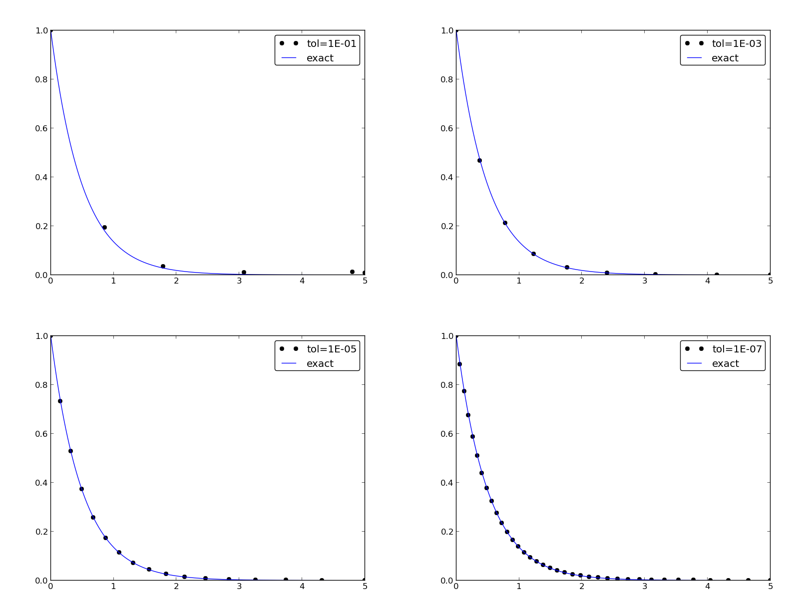
Computing convergence rates
Estimating the convergence rate $ r $
Brief implementation
We embed the code in a real test function
The manufactured solution can be computed by sympy
Execution
Debugging via convergence rates
Extension to systems of ODEs
The Backward Euler method gives a system of algebraic equations
Methods for general first-order ODEs
Generic form
The $ \theta $-rule
Implicit 2-step backward scheme
The Leapfrog scheme
The filtered Leapfrog scheme
2nd-order Runge-Kutta scheme
4th-order Runge-Kutta scheme
2nd-order Adams-Bashforth scheme
3rd-order Adams-Bashforth scheme
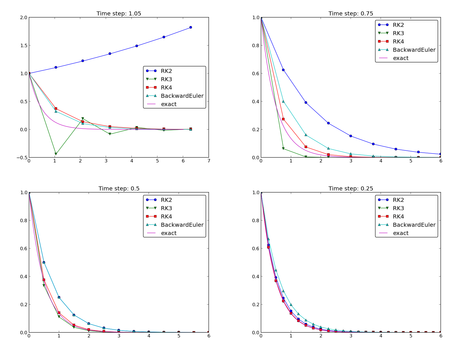
The Odespy software
Example: Runge-Kutta methods
Plots from the experiments
Example: Adaptive Runge-Kutta methods

Model extensions

Extension to a variable coefficient; Forward and Backward Euler

$$ \begin{equation} u'(t) = -a(t)u(t),\quad t\in (0,T],\quad u(0)=I \label{decay:problem:a} \end{equation} $$

The Forward Euler scheme: $$ \begin{equation} \frac{u^{n+1} - u^n}{\Delta t} = -a(t_n)u^n \label{_auto1} \end{equation} $$

The Backward Euler scheme: $$ \begin{equation} \frac{u^{n} - u^{n-1}}{\Delta t} = -a(t_n)u^n \label{_auto2} \end{equation} $$

Extension to a variable coefficient; Crank-Nicolson

Eevaluting $ a(t_{n+\half}) $ and using an average for $ u $: $$ \begin{equation} \frac{u^{n+1} - u^{n}}{\Delta t} = -a(t_{n+\half})\half(u^n + u^{n+1}) \label{_auto3} \end{equation} $$

Using an average for $ a $ and $ u $: $$ \begin{equation} \frac{u^{n+1} - u^{n}}{\Delta t} = -\half(a(t_n)u^n + a(t_{n+1})u^{n+1}) \label{_auto4} \end{equation} $$

Extension to a variable coefficient; $ \theta $-rule

The $ \theta $-rule unifies the three mentioned schemes, $$ \begin{equation} \frac{u^{n+1} - u^{n}}{\Delta t} = -a((1-\theta)t_n + \theta t_{n+1})((1-\theta) u^n + \theta u^{n+1}) \label{_auto5} \end{equation} $$ or, $$ \begin{equation} \frac{u^{n+1} - u^{n}}{\Delta t} = -(1-\theta) a(t_n)u^n - \theta a(t_{n+1})u^{n+1} \label{_auto6} \end{equation} $$

Extension to a variable coefficient; operator notation

$$ \begin{align*} \lbrack D^+_t u &= -au\rbrack^n,\\ \lbrack D^-_t u &= -au\rbrack^n,\\ \lbrack D_t u &= -a\overline{u}^t\rbrack^{n+\half},\\ \lbrack D_t u &= -\overline{au}^t\rbrack^{n+\half}\\ \end{align*} $$

Extension to a source term

$$ \begin{equation} u'(t) = -a(t)u(t) + b(t),\quad t\in (0,T],\quad u(0)=I \label{decay:problem:ab} \end{equation} $$ $$ \begin{align*} \lbrack D^+_t u &= -au + b\rbrack^n,\\ \lbrack D^-_t u &= -au + b\rbrack^n,\\ \lbrack D_t u &= -a\overline{u}^t + b\rbrack^{n+\half},\\ \lbrack D_t u &= \overline{-au+b}^t\rbrack^{n+\half} \end{align*} $$

Implementation of the generalized model problem

$$ \begin{equation} u^{n+1} = ((1 - \Delta t(1-\theta)a^n)u^n + \Delta t(\theta b^{n+1} + (1-\theta)b^n))(1 + \Delta t\theta a^{n+1})^{-1} \label{_auto7} \end{equation} $$

Implementation where $ a(t) $ and $ b(t) $ are given as Python functions (see file decay_vc.py):

def solver(I, a, b, T, dt, theta):
    """
    Solve u'=-a(t)*u + b(t), u(0)=I,
    for t in (0,T] with steps of dt.
    a and b are Python functions of t.
    """
    dt = float(dt)            # avoid integer division
    Nt = int(round(T/dt))     # no of time intervals
    T = Nt*dt                 # adjust T to fit time step dt
    u = zeros(Nt+1)           # array of u[n] values
    t = linspace(0, T, Nt+1)  # time mesh

    u[0] = I                  # assign initial condition
    for n in range(0, Nt):    # n=0,1,...,Nt-1
        u[n+1] = ((1 - dt*(1-theta)*a(t[n]))*u[n] + \ 
                  dt*(theta*b(t[n+1]) + (1-theta)*b(t[n])))/\ 
                  (1 + dt*theta*a(t[n+1]))
    return u, t

Implementations of variable coefficients; functions

Plain functions:

def a(t):
    return a_0 if t < tp else k*a_0

def b(t):
    return 1

Implementations of variable coefficients; classes

Better implementation: class with the parameters a0, tp, and k as attributes and a special method __call__ for evaluating $ a(t) $:

class A:
    def __init__(self, a0=1, k=2):
        self.a0, self.k = a0, k

    def __call__(self, t):
        return self.a0 if t < self.tp else self.k*self.a0

a = A(a0=2, k=1)  # a behaves as a function a(t)

Implementations of variable coefficients; lambda function

Quick writing: a one-liner lambda function

a = lambda t: a_0 if t < tp else k*a_0

In general,

f = lambda arg1, arg2, ...: expressin

is equivalent to

def f(arg1, arg2, ...):
    return expression

One can use lambda functions directly in calls:

u, t = solver(1, lambda t: 1, lambda t: 1, T, dt, theta)

for a problem $ u'=-u+1 $, $ u(0)=1 $.

A lambda function can appear anywhere where a variable can appear.

Verification via trivial solutions

Start debugging of a new code with trying a problem where $ u=\hbox{const} \neq 0 $.

Choose $ u=C $ (a constant). Choose any $ a(t) $ and set $ b=a(t)C $ and $ I=C $.

"All" numerical methods will reproduce $ u=_{\hbox{const}} $ exactly (machine precision).

Often $ u=C $ eases debugging.

In this example: any error in the formula for $ u^{n+1} $ make $ u\neq C $!

Verification via trivial solutions; test function

def test_constant_solution():
    """
    Test problem where u=u_const is the exact solution, to be
    reproduced (to machine precision) by any relevant method.
    """
    def u_exact(t):
        return u_const

    def a(t):
        return 2.5*(1+t**3)  # can be arbitrary

    def b(t):
        return a(t)*u_const

    u_const = 2.15
    theta = 0.4; I = u_const; dt = 4
    Nt = 4  # enough with a few steps
    u, t = solver(I=I, a=a, b=b, T=Nt*dt, dt=dt, theta=theta)
    print u
    u_e = u_exact(t)
    difference = abs(u_e - u).max()  # max deviation
    tol = 1E-14
    assert difference < tol

Verification via manufactured solutions

Choose any formula for $ u(t) $

Fit $ I $, $ a(t) $, and $ b(t) $ in $ u'=-au+b $, $ u(0)=I $, to make the chosen formula a solution of the ODE problem

Then we can always have an analytical solution (!)

Ideal for verification: testing convergence rates

Called the method of manufactured solutions (MMS)

Special case: $ u $ linear in $ t $, because all sound numerical methods will reproduce a linear $ u $ exactly (machine precision)

$ u(t) = ct + d $. $ u(0)=I $ means $ d=I $

ODE implies $ c = -a(t)u + b(t) $

Choose $ a(t) $ and $ c $, and set $ b(t) = c + a(t)(ct + I) $

Any error in the formula for $ u^{n+1} $ makes $ u\neq ct+I $!

Linear manufactured solution

$ u^n = ct_n+I $ fulfills the discrete equations!

First, $$ \begin{align} \lbrack D_t^+ t\rbrack^n &= \frac{t_{n+1}-t_n}{\Delta t}=1, \label{decay:fd2:Dop:tn:fw}\\ \lbrack D_t^- t\rbrack^n &= \frac{t_{n}-t_{n-1}}{\Delta t}=1, \label{decay:fd2:Dop:tn:bw}\\ \lbrack D_t t\rbrack^n &= \frac{t_{n+\half}-t_{n-\half}}{\Delta t}=\frac{(n+\half)\Delta t - (n-\half)\Delta t}{\Delta t}=1\label{decay:fd2:Dop:tn:cn} \end{align} $$

Forward Euler: $$ [D^+ u = -au + b]^n $$

$ a^n=a(t_n) $, $ b^n=c + a(t_n)(ct_n + I) $, and $ u^n=ct_n + I $ results in $$ c = -a(t_n)(ct_n+I) + c + a(t_n)(ct_n + I) = c $$

Test function for linear manufactured solution

def test_linear_solution():
    """
    Test problem where u=c*t+I is the exact solution, to be
    reproduced (to machine precision) by any relevant method.
    """
    def u_exact(t):
        return c*t + I

    def a(t):
        return t**0.5  # can be arbitrary

    def b(t):
        return c + a(t)*u_exact(t)

    theta = 0.4; I = 0.1; dt = 0.1; c = -0.5
    T = 4
    Nt = int(T/dt)  # no of steps
    u, t = solver(I=I, a=a, b=b, T=Nt*dt, dt=dt, theta=theta)
    u_e = u_exact(t)
    difference = abs(u_e - u).max()  # max deviation
    print difference
    tol = 1E-14  # depends on c!
    assert difference < tol

Computing convergence rates

Frequent assumption on the relation between the numerical error $ E $ and some discretization parameter $ \Delta t $: $$ \begin{equation} E = C\Delta t^r, \label{decay:E:dt} \end{equation} $$

Unknown: $ C $ and $ r $.

Goal: estimate $ r $ (and $ C $) from numerical experiments, by looking at consecutive pairs of $ (\Delta t_i, E_i) $ and $ (\Delta t_{i-1}, E_{i-1}) $.

Estimating the convergence rate $ r $

Perform numerical experiments: $ (\Delta t_i, E_i) $, $ i=0,\ldots,m-1 $. Two methods for finding $ r $ (and $ C $):

Take the logarithm of \eqref{decay:E:dt}, $ \ln E = r\ln \Delta t + \ln C $, and fit a straight line to the data points $ (\Delta t_i, E_i) $, $ i=0,\ldots,m-1 $.

Consider two consecutive experiments, $ (\Delta t_i, E_i) $ and $ (\Delta t_{i-1}, E_{i-1}) $. Dividing the equation $ E_{i-1}=C\Delta t_{i-1}^r $ by $ E_{i}=C\Delta t_{i}^r $ and solving for $ r $ yields

$$ \begin{equation} r_{i-1} = \frac{\ln (E_{i-1}/E_i)}{\ln (\Delta t_{i-1}/\Delta t_i)} \label{decay:conv:rate} \end{equation} $$ for $ i=1,=\ldots,m-1 $.

Method 2 is best.

Brief implementation

Compute $ r_0, r_1, \ldots, r_{m-2} $ from $ E_i $ and $ \Delta t_i $:

def compute_rates(dt_values, E_values):
    m = len(dt_values)
    r = [log(E_values[i-1]/E_values[i])/
         log(dt_values[i-1]/dt_values[i])
         for i in range(1, m, 1)]
    # Round to two decimals
    r = [round(r_, 2) for r_ in r]
    return r

We embed the code in a real test function

def test_convergence_rates():
    # Create a manufactured solution
    # define u_exact(t), a(t), b(t)

    dt_values = [0.1*2**(-i) for i in range(7)]
    I = u_exact(0)

    for theta in (0, 1, 0.5):
        E_values = []
        for dt in dt_values:
            u, t = solver(I=I, a=a, b=b, T=6, dt=dt, theta=theta)
            u_e = u_exact(t)
            e = u_e - u
            E = sqrt(dt*sum(e**2))
            E_values.append(E)
        r = compute_rates(dt_values, E_values)
        print 'theta=%g, r: %s' % (theta, r)
        expected_rate = 2 if theta == 0.5 else 1
        tol = 0.1
        diff = abs(expected_rate - r[-1])
        assert diff < tol

The manufactured solution can be computed by sympy

We choose $ \uex(t) = \sin(t)e^{-2t} $, $ a(t)=t^2 $, fit $ b(t)=u'(t)-a(t) $:

# Create a manufactured solution with sympy
import sympy as sym
t = sym.symbols('t')
u_exact = sym.sin(t)*sym.exp(-2*t)
a = t**2
b = sym.diff(u_exact, t) + a*u_exact

# Turn sympy expressions into Python function
u_exact = sym.lambdify([t], u_exact, modules='numpy')
a = sym.lambdify([t], a, modules='numpy')
b = sym.lambdify([t], b, modules='numpy')

Complete code: decay_vc.py.

Execution

Terminal> python decay_vc.py
...
theta=0, r: [1.06, 1.03, 1.01, 1.01, 1.0, 1.0]
theta=1, r: [0.94, 0.97, 0.99, 0.99, 1.0, 1.0]
theta=0.5, r: [2.0, 2.0, 2.0, 2.0, 2.0, 2.0]

Debugging via convergence rates

Potential bug: missing a in the denominator,

u[n+1] = (1 - (1-theta)*a*dt)/(1 + theta*dt)*u[n]

Running decay_convrate.py gives same rates.

Why? The value of $ a $... ($ a=1 $)

0 and 1 are bad values in tests!

Better:

Terminal> python decay_convrate.py --a 2.1 --I 0.1  \ 
          --dt 0.5 0.25 0.1 0.05 0.025 0.01
...
Pairwise convergence rates for theta=0:
1.49 1.18 1.07 1.04 1.02

Pairwise convergence rates for theta=0.5:
-1.42 -0.22 -0.07 -0.03 -0.01

Pairwise convergence rates for theta=1:
0.21 0.12 0.06 0.03 0.01

Forward Euler works...because $ \theta=0 $ hides the bug.

This bug gives $ r\approx 0 $:

u[n+1] = ((1-theta)*a*dt)/(1 + theta*dt*a)*u[n]

Extension to systems of ODEs

Sample system: $$ \begin{align} u' &= a u + bv \label{_auto8}\\ v' &= cu + dv \label{_auto9} \end{align} $$

The Forward Euler method: $$ \begin{align} u^{n+1} &= u^n + \Delta t (a u^n + b v^n) \label{_auto10}\\ v^{n+1} &= u^n + \Delta t (cu^n + dv^n) \label{_auto11} \end{align} $$

The Backward Euler method gives a system of algebraic equations

The Backward Euler scheme: $$ \begin{align} u^{n+1} &= u^n + \Delta t (a u^{n+1} + b v^{n+1}) \label{_auto12}\\ v^{n+1} &= v^n + \Delta t (c u^{n+1} + d v^{n+1}) \label{_auto13} \end{align} $$ which is a $ 2\times 2 $ linear system: $$ \begin{align} (1 - \Delta t a)u^{n+1} + bv^{n+1} &= u^n \label{_auto14}\\ c u^{n+1} + (1 - \Delta t d) v^{n+1} &= v^n \label{_auto15} \end{align} $$

Crank-Nicolson also gives a $ 2\times 2 $ linear system.

Methods for general first-order ODEs

Generic form

The standard form for ODEs: $$ \begin{equation} u' = f(u,t),\quad u(0)=I \label{decay:ode:general} \end{equation} $$

$ u $ and $ f $: scalar or vector.

Vectors in case of ODE systems: $$ u(t) = (u^{(0)}(t),u^{(1)}(t),\ldots,u^{(m-1)}(t)) $$ $$ \begin{align*} f(u, t) = ( & f^{(0)}(u^{(0)},\ldots,u^{(m-1)})\\ & f^{(1)}(u^{(0)},\ldots,u^{(m-1)}),\\ & \vdots\\ & f^{(m-1)}(u^{(0)}(t),\ldots,u^{(m-1)}(t))) \end{align*} $$

The $ \theta $-rule

$$ \begin{equation} \frac{u^{n+1}-u^n}{\Delta t} = \theta f(u^{n+1},t_{n+1}) + (1-\theta)f(u^n, t_n) \label{decay:fd2:theta} \end{equation} $$ Bringing the unknown $ u^{n+1} $ to the left-hand side and the known terms on the right-hand side gives $$ \begin{equation} u^{n+1} - \Delta t \theta f(u^{n+1},t_{n+1}) = u^n + \Delta t(1-\theta)f(u^n, t_n) \label{_auto16} \end{equation} $$ This is a nonlinear equation in $ u^{n+1} $ (unless $ f $ is linear in $ u $)!

Implicit 2-step backward scheme

$$ u'(t_{n+1}) \approx \frac{3u^{n+1} - 4u^{n} + u^{n-1}}{2\Delta t}$$

Scheme: $$ u^{n+1} = \frac{4}{3}u^n - \frac{1}{3}u^{n-1} + \frac{2}{3}\Delta t f(u^{n+1}, t_{n+1}) \label{decay:fd2:bw:2step} $$ Nonlinear equation for $ u^{n+1} $.

The Leapfrog scheme

Idea: $$ \begin{equation} u'(t_n)\approx \frac{u^{n+1}-u^{n-1}}{2\Delta t} = [D_{2t} u]^n \label{_auto17} \end{equation} $$

Scheme: $$ [D_{2t} u = f(u,t)]^n$$ or written out, $$ \begin{equation} u^{n+1} = u^{n-1} + 2 \Delta t f(u^n, t_n) \label{decay:fd2:leapfrog} \end{equation} $$

Some other scheme must be used as starter ($ u^1 $).

Explicit scheme - a nonlinear $ f $ (in $ u $) is trivial to handle.

Downside: Leapfrog is always unstable after some time.

The filtered Leapfrog scheme

After computing $ u^{n+1} $, stabilize Leapfrog by $$ \begin{equation} u^n\ \leftarrow\ u^n + \gamma (u^{n-1} - 2u^n + u^{n+1}) \label{decay:fd2:leapfrog:filtered} \end{equation} $$

2nd-order Runge-Kutta scheme

Forward-Euler + approximate Crank-Nicolson: $$ \begin{align} u^* &= u^n + \Delta t f(u^n, t_n), \label{decay:fd2:RK2:s1}\\ u^{n+1} &= u^n + \Delta t \half \left( f(u^n, t_n) + f(u^*, t_{n+1}) \right) \label{decay:fd2:RK2:s2} \end{align} $$

4th-order Runge-Kutta scheme

The most famous and widely used ODE method

4 evaluations of $ f $ per time step

Its derivation is a very good illustration of numerical thinking!

2nd-order Adams-Bashforth scheme

$$ \begin{equation} u^{n+1} = u^n + \half\Delta t\left( 3f(u^n, t_n) - f(u^{n-1}, t_{n-1}) \right) \label{decay:fd2:AB2} \end{equation} $$

3rd-order Adams-Bashforth scheme

$$ \begin{equation} u^{n+1} = u^n + \frac{1}{12}\left( 23f(u^n, t_n) - 16 f(u^{n-1},t_{n-1}) + 5f(u^{n-2}, t_{n-2})\right) \label{decay:fd2:AB3} \end{equation} $$

The Odespy software

Odespy features simple Python implementations of the most fundamental schemes as well as Python interfaces to several famous packages for solving ODEs: ODEPACK, Vode, rkc.f, rkf45.f, Radau5, as well as the ODE solvers in SciPy, SymPy, and odelab.

Typical usage:

# Define right-hand side of ODE
def f(u, t):
    return -a*u

import odespy
import numpy as np

# Set parameters and time mesh
I = 1; a = 2; T = 6; dt = 1.0
Nt = int(round(T/dt))
t_mesh = np.linspace(0, T, Nt+1)

# Use a 4th-order Runge-Kutta method
solver = odespy.RK4(f)
solver.set_initial_condition(I)
u, t = solver.solve(t_mesh)

Example: Runge-Kutta methods

solvers = [odespy.RK2(f),
           odespy.RK3(f),
           odespy.RK4(f),
           odespy.BackwardEuler(f, nonlinear_solver='Newton')]

for solver in solvers:
    solver.set_initial_condition(I)
    u, t = solver.solve(t)

# + lots of plot code...

Plots from the experiments

The 4-th order Runge-Kutta method (RK4) is the method of choice!

Example: Adaptive Runge-Kutta methods

Adaptive methods find "optimal" locations of the mesh points to ensure that the error is less than a given tolerance.

Downside: approximate error estimation, not always optimal location of points.

"Industry standard ODE solver": Dormand-Prince 4/5-th order Runge-Kutta (MATLAB's famous ode45).