$$
\newcommand{\half}{\frac{1}{2}}
\newcommand{\tp}{\thinspace .}
\newcommand{\uex}{{u_{\small\mbox{e}}}}
\newcommand{\Aex}{{A_{\small\mbox{e}}}}
\newcommand{\E}[1]{\hbox{E}\lbrack #1 \rbrack}
\newcommand{\Var}[1]{\hbox{Var}\lbrack #1 \rbrack}
\newcommand{\Std}[1]{\hbox{Std}\lbrack #1 \rbrack}
\newcommand{\Oof}[1]{\mathcal{O}(#1)}
\newcommand{\stress}{\boldsymbol{\sigma}}
$$
Summarizing multiple-choice questions
Quiz
Exercise 6.1: Characterize a finite difference
Question: We can approximate the derivative at a point using two function values:
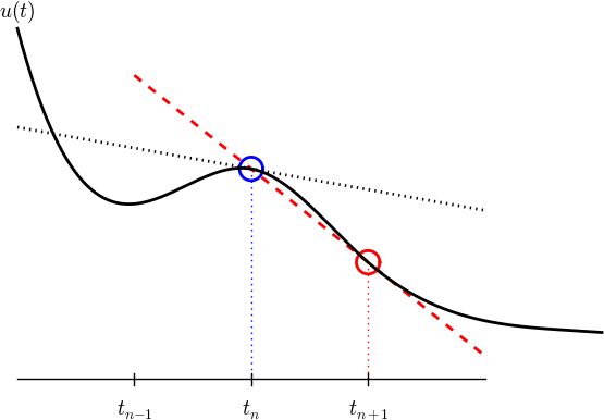
What is this type of difference called and how large is the error?
Choice A:
This is a centered difference with error proportional to \( \Delta t^2 \).
Choice B:
This is a forward difference with error proportional to \( \Delta t \).
Choice C:
This is a Forward Euler difference with error proportional to \( \Delta t^3 \).
Choice D:
This is a Backward Euler finite difference with error proportional to \( \Delta t \).
Exercise 6.2: Characterize a finite difference
Question: We can approximate the derivative at a point using two function values:
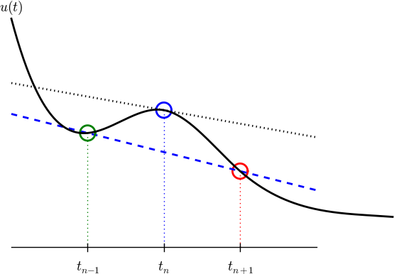
What is this type of difference called and how large is the error?
Choice A:
This is a centered difference with error proportional to \( \Delta t^2 \).
Choice B:
This is a forward difference with error proportional to \( \Delta t^2 \).
Choice C:
This is a centered difference with error proportional to \( \Delta t^4 \).
Choice D:
This is a Backward Euler finite difference with error proportional to \( \Delta t \).
Exercise 6.3: What is the problem with this program?
Question: We want to solve
$$ u ' = -au, \quad u(0)=1, $$
by a Forward Euler scheme,
$$ u^{n+1} = u^n - a\Delta t\, u^n,$$
and the following program
from numpy import *
u = zeros(10)
u[0] = 1
dt = 0.1
for i in range(10):
    u[i+1] = u[i] - dt*a*u[n]
What is the major problem with this program?
Choice A:
from numpy import * is not recommended; one should import explicitly the functions needed or do import numpy as np.
Choice B:
The program aborts with a NameError.
Choice C:
The program is "flat". It should be wrapped in a function solver(U0, dt, N, a).
Choice D:
The scheme is unstable!
Exercise 6.4: Is the solution correct?
Question: You have solved \( u'=-au \) by the Crank-Nicolson scheme and tested
your program thoroughly. Suddenly you run the program with \( I=1 \), \( a=10 \), \( T=1 \), and \( \Delta t=0.225 \). You get somewhat unexpected results:
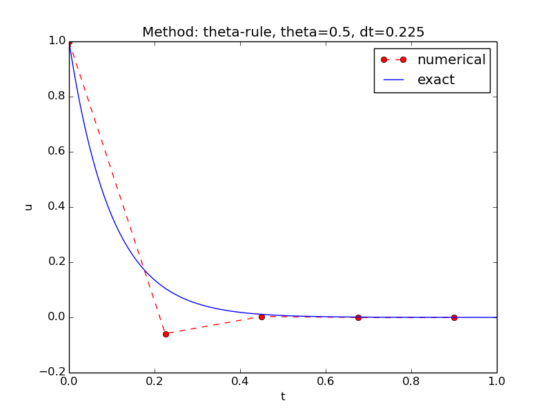
The results are unexpected because we know the exact solution should be
monotone and decreasing, while this numerical solution also shows an
increasing stage. What is the problem?
Choice A:
The program is not tested well enough - yet another bug is there.
Choice B:
The numerical solution method is more general than the analytical one,
and this is an example where the solution can increase, but the analytical
solution technique is not capable of dealing with this situation.
Choice C:
The time step is too large and cause an instability in the form of non-physical oscillations.
Choice D:
The Crank-Nicolson scheme is unconditionally stable and can be used with all time-step sizes, but the problem here is that round-off errors due to a "too large" \( a \) (10, not around 1) accumulate to the effect seen in the plot.
Exercise 6.5: Is this a proper test function?
Question: Suppose we have some function compute that we want to test. We construct
a unit test and implement an associated test function (according to the
rules for test functions in the nose or pytest test frameworks):
def test_compute(n):
    expected = (n**2)/4.5 - 1
    computed = compute(n)
    assert expected != computed
The question is if this test function can be used as is or if improvements
must be implemented.
Choice A:
One should use special assert functions from nose.tools, here the choice is nose.tools.assert_almost_equal.
Choice B:
One cannot test compute(n) for only one n value. Many are required for good evidence that the function works.
Choice C:
The test function does not test expected != computed with a tolerance
and the n parameter cannot be an argument.
Choice D:
The assert statement also needs a message explaining what is wrong when the test fails.
Exercise 6.6: Rewrite an expression with array arithmetics
Question: A mesh function is initialized with the code segment
from math import exp
N_t = 100
T = 3.0
dt = T/N_t
t = []
u = []
for i in range(len(t)):
    t.append(i*dt)
    u.append(1 - exp(-t[-1]))
Rewrite this code such that there is no loop and u is computed by
array arithmetics.
Choice A:
from numpy import *
from math import exp
N_t = 100
t = np.linspace(0, 3, N_t+1)
u = 1 - exp(-t)
Choice B:
import numpy as np
N_t = 100
t = np.linspace(0, 3, N_t+1)
u = 1 - np.exp(-t)
Choice C:
N_t = 100
dt = 3.0/N_t
t = [i*dt for i in range(N_t+1)]
from numpy import exp
u = 1 - exp(-t)
Choice D:
import numpy
t = numpy.mesh([0, 3], 100)
u = numpy.func(numpy.exp, t)
Exercise 6.7: What is the truncation error?
Question: What is the truncation error?
Choice A:
The difference between the exact solution and the numerical solution
at a mesh point.
Choice B:
The error in the factor that takes u[i] to u[i+1].
Choice C:
The difference between the exact solution and the numerical
solution truncated to one decimal.
Choice D:
The error in the scheme when the exact solution is inserted in the
scheme's difference equation.
Exercise 6.8: Recognize a programming language
Question: What kind of programming language is this?
function integral = trapezoidal(f, a, b, n)
    %% Integrate f from a to b with n intervals
    h = (b-a)/n;
    result = 0.5*f(a) + 0.5*f(b);
    for i = 1:(n-1)
        result = result + f(a + i*h);
    end
    integral = h*result;
end
Choice A:
Python
Choice B:
MATLAB or Octave
Choice C:
Cython
Choice D:
FORTRAN 77
Exercise 6.9: Recognize a programming language
Question: What kind of programming language is this?
def trapezoidal(f, a, b, n):
    # Integrate f from a to b with n intervals
    h = (b-a)/float(n)
    result = 0.5*f(a) + 0.5*f(b)
    for i in range(1, n):
        result += f(a + i*h)
    return h*result
Choice A:
Python
Choice B:
MATLAB or Octave
Choice C:
Cython
Choice D:
FORTRAN 77
Exercise 6.10: Recognize a programming language
Question: What kind of programming language is this?
      real*8 function trapezoidal(f, a, b, n)
C     Integrate f from a to b with n intervals
      real*8 h, result, f
      external f
      h = (b-a)/n
      result = 0.5*f(a) + 0.5*f(b)
      do i = 1, n-1
        result = result + f(a + i*h)
      end do
      trapezoidal = h*result
      return
      end
Choice A:
Python
Choice B:
MATLAB or Octave
Choice C:
Cython
Choice D:
FORTRAN 77
Exercise 6.11: Recognize a programming language
Question: What kind of programming language is this?
double trapezoidal(
    double (*f)(double), double a, double b, int n)
{
    double h, result;
    h = (b-a)/n;
    result = 0.5*f(a) + 0.5*f(b);
    for (i=1; i++; i <= n-1) {
        result += f(a + i*h);
    }
    return h*result;
}
Choice A:
C
Choice B:
C++
Choice C:
Cython
Choice D:
Octave dialect
Exercise 6.12: What is SymPy?
Question: What is SymPy?
Choice A:
A Python module for computing with symmetric matrices.
Choice B:
A Python package for doing symbolic computations (exact/analytical differentiation, integration, equation solves, etc.).
Choice C:
A Python package for numerical approximations to differentiation, integration, equation solving, etc.
Choice D:
A free, open source version of Mathematica.
Exercise 6.13: Testing of code
Question: What is an appropriate test for computing the solution of some ODE?
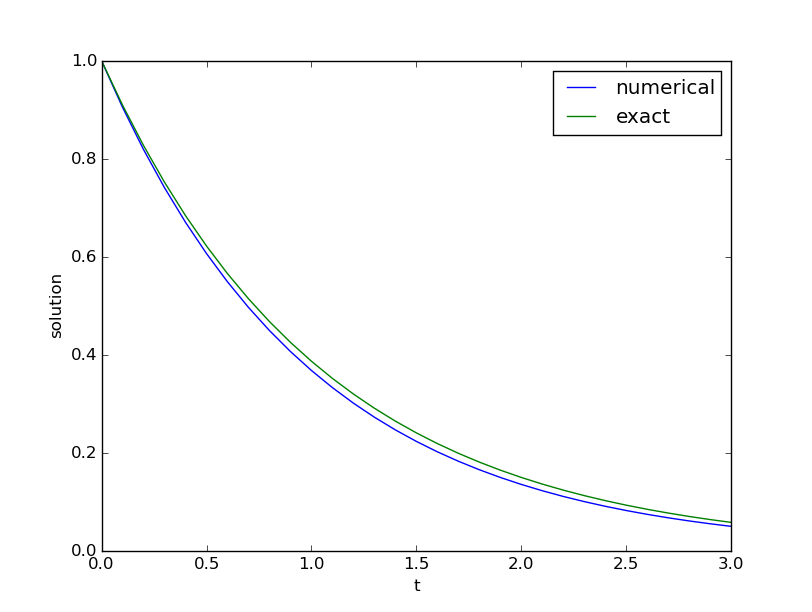
Choice A:
We compare the numerical solution with the analytical solution
in a plot. The curves are quite close, showing that the computations
are correct (here using 31 mesh points).
Choice B:
The maximum error between the numerical and exact solution at
the mesh points is \( 1.886\cdot 10^{-5} \), which is small. Therefore, the
program works.
Choice C:
The scheme is \( \Oof{\Delta t^2} \). With 31 points we get a maximum
point-wise error of \( 1.243\cdot 10^{-4} \). With 61 points (halving \( \Delta t \))
the corresponding error is \( 3.108\cdot 10^{-5} \). This is a reduction of
approximately a factor 4, which is what we expect for such a scheme when
halving \( \Delta t \).
Choice D:
The numerical solution and the exact solutions get closer and closer
in a plot as we reduce \( \Delta t \). Therefore, the program works.
Exercise 6.14: What kind of scheme is this?
Question: Given \( u^{\prime}=-au + b \), where \( a \) and \( b \) are functions of time.
Is the following scheme correct?
$$ \frac{u^{n}-u^{n-1}}{\Delta t} = -a(t_n)\frac{1}{2}(u^n + u^{n-1})
+ b(t_n)\tp$$
Choice A:
Yes, it is a Crank-Nicolson type of scheme.
Choice B:
Yes, if \( a(t_n) \) and \( b(t_n) \) are evaluated at the previous time
step, \( a(t_{n-1}) \) and \( a(t_{n-1}) \).
Choice C:
No, the coefficients \( a \) and \( b \) are not evaluated correctly.
Choice D:
No, the right-hand side should be \( a(t_n)u^n + b(t_n) \).
Exercise 6.15: What kind of scheme is this?
Question: We want to solve \( y'=g(x, y) \) for \( y(x) \) and have the scheme
$$ y^{i+1} = y^i + \Delta t\, g(x_{i+1}, y^{i+1})\tp$$
What is this scheme called?
Choice A:
The implicit midpoint scheme.
Choice B:
The Backward Euler scheme or just the backward scheme.
Choice C:
The Forward Euler scheme, Euler's method, or just the forward scheme.
Choice D:
The implicit Adams scheme of order one.
Exercise 6.16: What kind of scheme is this?
Question: We want to solve \( y'=g(x, y) \) for \( y(x) \) and have the scheme
$$ y^{i+1} = y^{i-1} + 2\Delta t\, g(x_{i}, y^{i})\tp$$
What is this scheme called?
Choice A:
The implicit midpoint scheme.
Choice B:
The two-step backward scheme.
Choice C:
The Crank-Nicolson scheme.
Choice D:
The leapfrog scheme.