$$ \newcommand{\half}{\frac{1}{2}} \newcommand{\uex}{{u_{\small\mbox{e}}}} \newcommand{\Aex}{{A_{\small\mbox{e}}}} \newcommand{\Oof}[1]{\mathcal{O}(#1)} $$

Study guide: Analysis of exponential decay models

Hans Petter Langtangen [1, 2]

[1] Center for Biomedical Computing, Simula Research Laboratory [2] Department of Informatics, University of Oslo

Sep 13, 2016

Analysis of finite difference equations
Encouraging numerical solutions
Discouraging numerical solutions; Crank-Nicolson
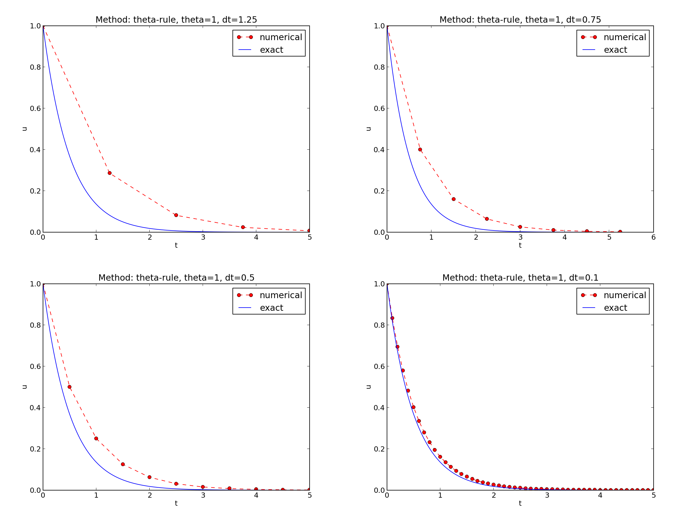
Discouraging numerical solutions; Forward Euler
Summary of observations
Problem setting
Experimental investigation of oscillatory solutions
Exact numerical solution
Stability
Computation of stability in this problem
Computation of stability in this problem
Explanation of problems with Forward Euler
Explanation of problems with Crank-Nicolson
Summary of stability
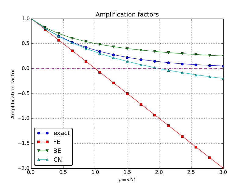
Comparing amplification factors
Plot of amplification factors
$ p=a\Delta t $ is the important parameter for numerical performance
Series expansion of amplification factors
Error in amplification factors
The fraction of numerical and exact amplification factors
The true/global error at a point
Computing the global error at a point
Convergence
Integrated errors
Truncation error
Computation of the truncation error
The truncation error for other schemes
Consistency, stability, and convergence

Analysis of finite difference equations

Model: $$ \begin{equation} u'(t) = -au(t),\quad u(0)=I \label{_auto1} \end{equation} $$

Method: $$ \begin{equation} u^{n+1} = \frac{1 - (1-\theta) a\Delta t}{1 + \theta a\Delta t}u^n \label{decay:analysis:scheme} \end{equation} $$

Problem setting.

How good is this method? Is it safe to use it?

Encouraging numerical solutions

$ I=1 $, $ a=2 $, $ \theta =1,0.5, 0 $, $ \Delta t=1.25, 0.75, 0.5, 0.1 $.

Discouraging numerical solutions; Crank-Nicolson

Discouraging numerical solutions; Forward Euler

Summary of observations

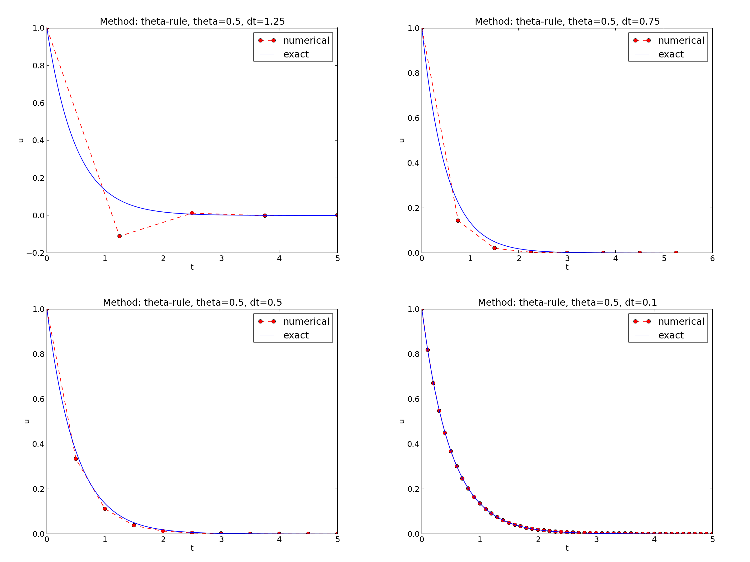
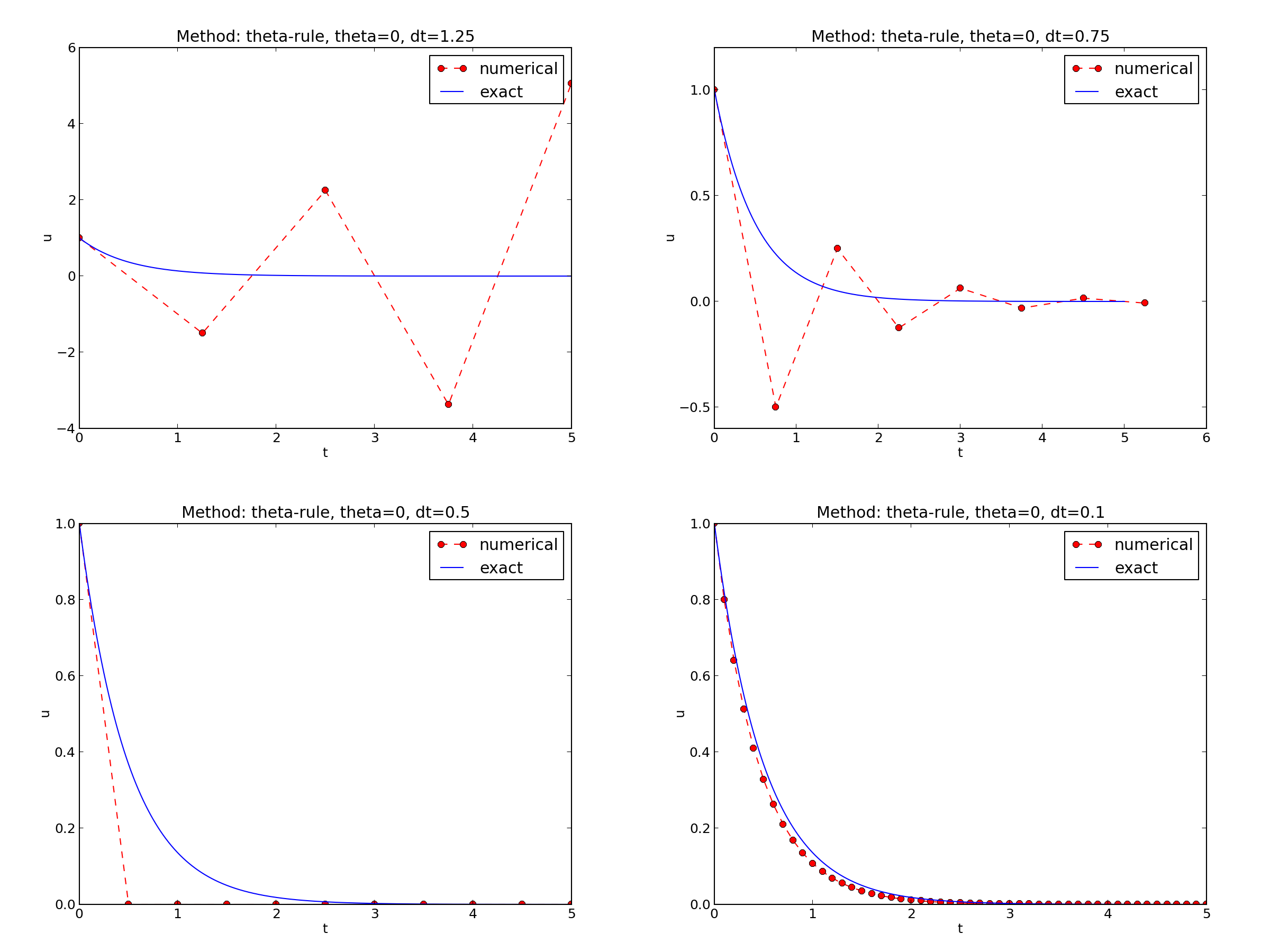
The characteristics of the displayed curves can be summarized as follows:

The Backward Euler scheme always gives a monotone solution, lying above the exact solution.

The Crank-Nicolson scheme gives the most accurate results, but for $ \Delta t=1.25 $ the solution oscillates.

The Forward Euler scheme gives a growing, oscillating solution for $ \Delta t=1.25 $; a decaying, oscillating solution for $ \Delta t=0.75 $; a strange solution $ u^n=0 $ for $ n\geq 1 $ when $ \Delta t=0.5 $; and a solution seemingly as accurate as the one by the Backward Euler scheme for $ \Delta t = 0.1 $, but the curve lies below the exact solution.

Problem setting

Goal.

We ask the question

Under what circumstances, i.e., values of the input data $ I $, $ a $, and $ \Delta t $ will the Forward Euler and Crank-Nicolson schemes result in undesired oscillatory solutions?

Techniques of investigation:

Numerical experiments

Mathematical analysis

Another question to be raised is

How does $ \Delta t $ impact the error in the numerical solution?

Experimental investigation of oscillatory solutions

The solution is oscillatory if $$ u^{n} > u^{n-1}$$ ("Safe choices" of $ \Delta t $ lie under the following curve as a function of $ a $.)

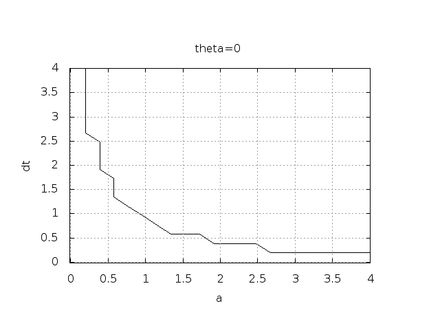
Seems that $ a\Delta t < 1 $ for FE and 2 for CN.

Exact numerical solution

Starting with $ u^0=I $, the simple recursion \eqref{decay:analysis:scheme} can be applied repeatedly $ n $ times, with the result that $$ \begin{equation} u^{n} = IA^n,\quad A = \frac{1 - (1-\theta) a\Delta t}{1 + \theta a\Delta t} \label{decay:analysis:unex} \end{equation} $$

Such a formula for the exact discrete solution is unusual to obtain in practice, but very handy for our analysis here.

Note: An exact dicrete solution fulfills a discrete equation (without round-off errors), whereas an exact solution fulfills the original mathematical equation.

Stability

Since $ u^n=I A^n $,

$ A < 0 $ gives a factor $ (-1)^n $ and oscillatory solutions

$ |A|>1 $ gives growing solutions

Recall: the exact solution is monotone and decaying

If these qualitative properties are not met, we say that the numerical solution is unstable

Computation of stability in this problem

$ A < 0 $ if $$ \frac{1 - (1-\theta) a\Delta t}{1 + \theta a\Delta t} < 0 $$ To avoid oscillatory solutions we must have $ A> 0 $ and $$ \begin{equation} \Delta t < \frac{1}{(1-\theta)a}\ \label{_auto2} \end{equation} $$

Always fulfilled for Backward Euler

$ \Delta t \leq 1/a $ for Forward Euler

$ \Delta t \leq 2/a $ for Crank-Nicolson

Computation of stability in this problem

$ |A|\leq 1 $ means $ -1\leq A\leq 1 $ $$ \begin{equation} -1\leq\frac{1 - (1-\theta) a\Delta t}{1 + \theta a\Delta t} \leq 1 \label{decay:th:stability} \end{equation} $$ $ -1 $ is the critical limit (because $ A\le 1 $ is always satisfied): $$ \begin{align*} \Delta t &\leq \frac{2}{(1-2\theta)a},\quad \mbox{when }\theta < \half \end{align*} $$

Always fulfilled for Backward Euler and Crank-Nicolson

$ \Delta t \leq 2/a $ for Forward Euler

Explanation of problems with Forward Euler

$ a\Delta t= 2\cdot 1.25=2.5 $ and $ A=-1.5 $: oscillations and growth

$ a\Delta t = 2\cdot 0.75=1.5 $ and $ A=-0.5 $: oscillations and decay

$ \Delta t=0.5 $ and $ A=0 $: $ u^n=0 $ for $ n>0 $

Smaller $ \Delta t $: qualitatively correct solution

Explanation of problems with Crank-Nicolson

$ \Delta t=1.25 $ and $ A=-0.25 $: oscillatory solution

Never any growing solution

Summary of stability

Forward Euler is conditionally stable

$ \Delta t < 2/a $ for avoiding growth

$ \Delta t\leq 1/a $ for avoiding oscillations

The Crank-Nicolson is unconditionally stable wrt growth and conditionally stable wrt oscillations

$ \Delta t < 2/a $ for avoiding oscillations

Backward Euler is unconditionally stable

Comparing amplification factors

$ u^{n+1} $ is an amplification $ A $ of $ u^n $: $$ u^{n+1} = Au^n,\quad A = \frac{1 - (1-\theta) a\Delta t}{1 + \theta a\Delta t} $$

The exact solution is also an amplification: $$ u(t_{n+1}) = \Aex u(t_n), \quad \Aex = e^{-a\Delta t}$$

A possible measure of accuracy: $ \Aex - A $

Plot of amplification factors

$ p=a\Delta t $ is the important parameter for numerical performance

$ p=a\Delta t $ is a dimensionless parameter

all expressions for stability and accuracy involve $ p $

Note that $ \Delta t $ alone is not so important, it is the combination with $ a $ through $ p=a\Delta t $ that matters

Another "proof" why $ p=a\Delta t $ is key.

If we scale the model by $ \bar t=at $, $ \bar u=u/I $, we get $ d\bar u/d\bar t = -\bar u $, $ \bar u(0)=1 $ (no physical parameters!). The analysis show that $ \Delta \bar t $ is key, corresponding to $ a\Delta t $ in the unscaled model.

Series expansion of amplification factors

To investigate $ \Aex - A $ mathematically, we can Taylor expand the expression, using $ p=a\Delta t $ as variable.

1 2 3 4 5 6 7 8 9 10 11 12 13 14 15 16 17 18 19 20 21 22
>>> from sympy import * >>> # Create p as a mathematical symbol with name 'p' >>> p = Symbol('p') >>> # Create a mathematical expression with p >>> A_e = exp(-p) >>> >>> # Find the first 6 terms of the Taylor series of A_e >>> A_e.series(p, 0, 6) 1 + (1/2)*p**2 - p - 1/6*p**3 - 1/120*p**5 + (1/24)*p**4 + O(p**6) >>> theta = Symbol('theta') >>> A = (1-(1-theta)*p)/(1+theta*p) >>> FE = A_e.series(p, 0, 4) - A.subs(theta, 0).series(p, 0, 4) >>> BE = A_e.series(p, 0, 4) - A.subs(theta, 1).series(p, 0, 4) >>> half = Rational(1,2) # exact fraction 1/2 >>> CN = A_e.series(p, 0, 4) - A.subs(theta, half).series(p, 0, 4) >>> FE (1/2)*p**2 - 1/6*p**3 + O(p**4) >>> BE -1/2*p**2 + (5/6)*p**3 + O(p**4) >>> CN (1/12)*p**3 + O(p**4)

Error in amplification factors

Focus: the error measure $ A-\Aex $ as function of $ \Delta t $ (recall that $ p=a\Delta t $): $$ \begin{equation} A-\Aex = \left\lbrace\begin{array}{ll} \Oof{\Delta t^2}, & \hbox{Forward and Backward Euler},\\ \Oof{\Delta t^3}, & \hbox{Crank-Nicolson} \end{array}\right. \label{_auto3} \end{equation} $$

The fraction of numerical and exact amplification factors

Focus: the error measure $ 1-A/\Aex $ as function of $ p=a\Delta t $:

1 2 3 4 5 6 7 8 9
>>> FE = 1 - (A.subs(theta, 0)/A_e).series(p, 0, 4) >>> BE = 1 - (A.subs(theta, 1)/A_e).series(p, 0, 4) >>> CN = 1 - (A.subs(theta, half)/A_e).series(p, 0, 4) >>> FE (1/2)*p**2 + (1/3)*p**3 + O(p**4) >>> BE -1/2*p**2 + (1/3)*p**3 + O(p**4) >>> CN (1/12)*p**3 + O(p**4)

Same leading-order terms as for the error measure $ A-\Aex $.

The true/global error at a point

The error in $ A $ reflects the local (amplification) error when going from one time step to the next

What is the global (true) error at $ t_n $? $ e^n = \uex(t_n) - u^n = Ie^{-at_n} - IA^n $

Taylor series expansions of $ e^n $ simplify the expression

Computing the global error at a point

1 2 3 4 5 6 7 8 9 10 11 12
>>> n = Symbol('n') >>> u_e = exp(-p*n) # I=1 >>> u_n = A**n # I=1 >>> FE = u_e.series(p, 0, 4) - u_n.subs(theta, 0).series(p, 0, 4) >>> BE = u_e.series(p, 0, 4) - u_n.subs(theta, 1).series(p, 0, 4) >>> CN = u_e.series(p, 0, 4) - u_n.subs(theta, half).series(p, 0, 4) >>> FE (1/2)*n*p**2 - 1/2*n**2*p**3 + (1/3)*n*p**3 + O(p**4) >>> BE (1/2)*n**2*p**3 - 1/2*n*p**2 + (1/3)*n*p**3 + O(p**4) >>> CN (1/12)*n*p**3 + O(p**4)

Substitute $ n $ by $ t/\Delta t $:

Forward and Backward Euler: leading order term $ \half ta^2\Delta t $

Crank-Nicolson: leading order term $ \frac{1}{12}ta^3\Delta t^2 $

Convergence

The numerical scheme is convergent if the global error $ e^n\rightarrow 0 $ as $ \Delta t\rightarrow 0 $. If the error has a leading order term $ \Delta t^r $, the convergence rate is of order $ r $.

Integrated errors

Focus: norm of the numerical error $$ ||e^n||_{\ell^2} = \sqrt{\Delta t\sum_{n=0}^{N_t} ({\uex}(t_n) - u^n)^2}$$

Forward and Backward Euler: $$ ||e^n||_{\ell^2} = \frac{1}{4}\sqrt{\frac{T^3}{3}} a^2\Delta t$$

Crank-Nicolson: $$ ||e^n||_{\ell^2} = \frac{1}{12}\sqrt{\frac{T^3}{3}}a^3\Delta t^2$$

Summary of errors.

Analysis of both the pointwise and the time-integrated true errors:

1st order for Forward and Backward Euler

2nd order for Crank-Nicolson

Truncation error

How good is the discrete equation?

Possible answer: see how well $ \uex $ fits the discrete equation

$$ \lbrack D^{+}_t u = -au\rbrack^n$$ i.e., $$ \frac{u^{n+1}-u^n}{\Delta t} = -au^n$$ Insert $ \uex $ (which does not in general fulfill this discrete equation): $$ \begin{equation} \frac{\uex(t_{n+1})-\uex(t_n)}{\Delta t} + a\uex(t_n) = R^n \neq 0 \label{decay:analysis:trunc:Req} \end{equation} $$

Computation of the truncation error

The residual $ R^n $ is the truncation error.

How does $ R^n $ vary with $ \Delta t $?

Tool: Taylor expand $ \uex $ around the point where the ODE is sampled (here $ t_n $) $$ \uex(t_{n+1}) = \uex(t_n) + \uex'(t_n)\Delta t + \half\uex''(t_n) \Delta t^2 + \cdots $$ Inserting this Taylor series in \eqref{decay:analysis:trunc:Req} gives $$ R^n = \uex'(t_n) + \half\uex''(t_n)\Delta t + \ldots + a\uex(t_n)$$ Now, $ \uex $ solves the ODE $ \uex'=-a\uex $, and then $$ R^n \approx \half\uex''(t_n)\Delta t$$ This is a mathematical expression for the truncation error.

The truncation error for other schemes

Backward Euler: $$ R^n \approx -\half\uex''(t_n)\Delta t $$

Crank-Nicolson: $$ R^{n+\half} \approx \frac{1}{24}\uex'''(t_{n+\half})\Delta t^2$$

Consistency, stability, and convergence

Truncation error measures the residual in the difference equations. The scheme is consistent if the truncation error goes to 0 as $ \Delta t\rightarrow 0 $. Importance: the difference equations approaches the differential equation as $ \Delta t\rightarrow 0 $.

Stability means that the numerical solution exhibits the same qualitative properties as the exact solution. Here: monotone, decaying function.

Convergence implies that the true (global) error $ e^n =\uex(t_n)-u^n\rightarrow 0 $ as $ \Delta t\rightarrow 0 $. This is really what we want!

The Lax equivalence theorem for linear differential equations: consistency + stability is equivalent with convergence.

(Consistency and stability is in most problems much easier to establish than convergence.)

Study guide: Analysis of exponential decay models

Sep 13, 2016

Table of contents

Analysis of finite difference equations

Encouraging numerical solutions

Discouraging numerical solutions; Crank-Nicolson

Discouraging numerical solutions; Forward Euler

Summary of observations

Problem setting

Experimental investigation of oscillatory solutions

Exact numerical solution

Stability

Computation of stability in this problem

Computation of stability in this problem

Explanation of problems with Forward Euler

Explanation of problems with Crank-Nicolson

Summary of stability

Comparing amplification factors

Plot of amplification factors

\( p=a\Delta t \) is the important parameter for numerical performance

Series expansion of amplification factors

Error in amplification factors

The fraction of numerical and exact amplification factors

The true/global error at a point

Computing the global error at a point

Convergence

Integrated errors

Truncation error

Computation of the truncation error

The truncation error for other schemes

Consistency, stability, and convergence