Study guide: Analysis of exponential decay models
Sep 13, 2016
Analysis of finite difference equations
Model:
$$
\begin{equation}
u'(t) = -au(t),\quad u(0)=I
\tag{1}
\end{equation}
$$
Method:
$$
\begin{equation}
u^{n+1} = \frac{1 - (1-\theta) a\Delta t}{1 + \theta a\Delta t}u^n
\tag{2}
\end{equation}
$$
How good is this method? Is it safe to use it?
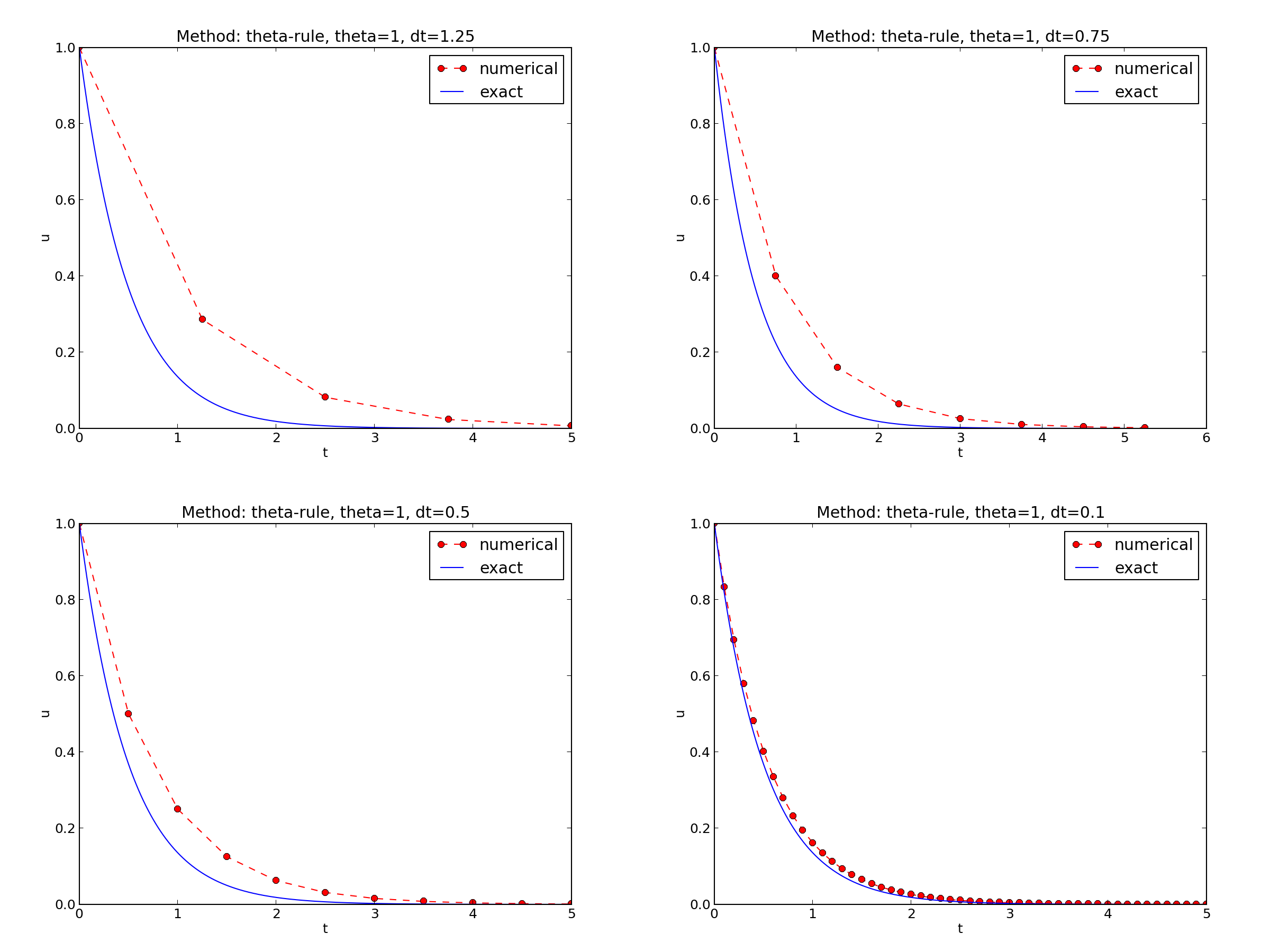
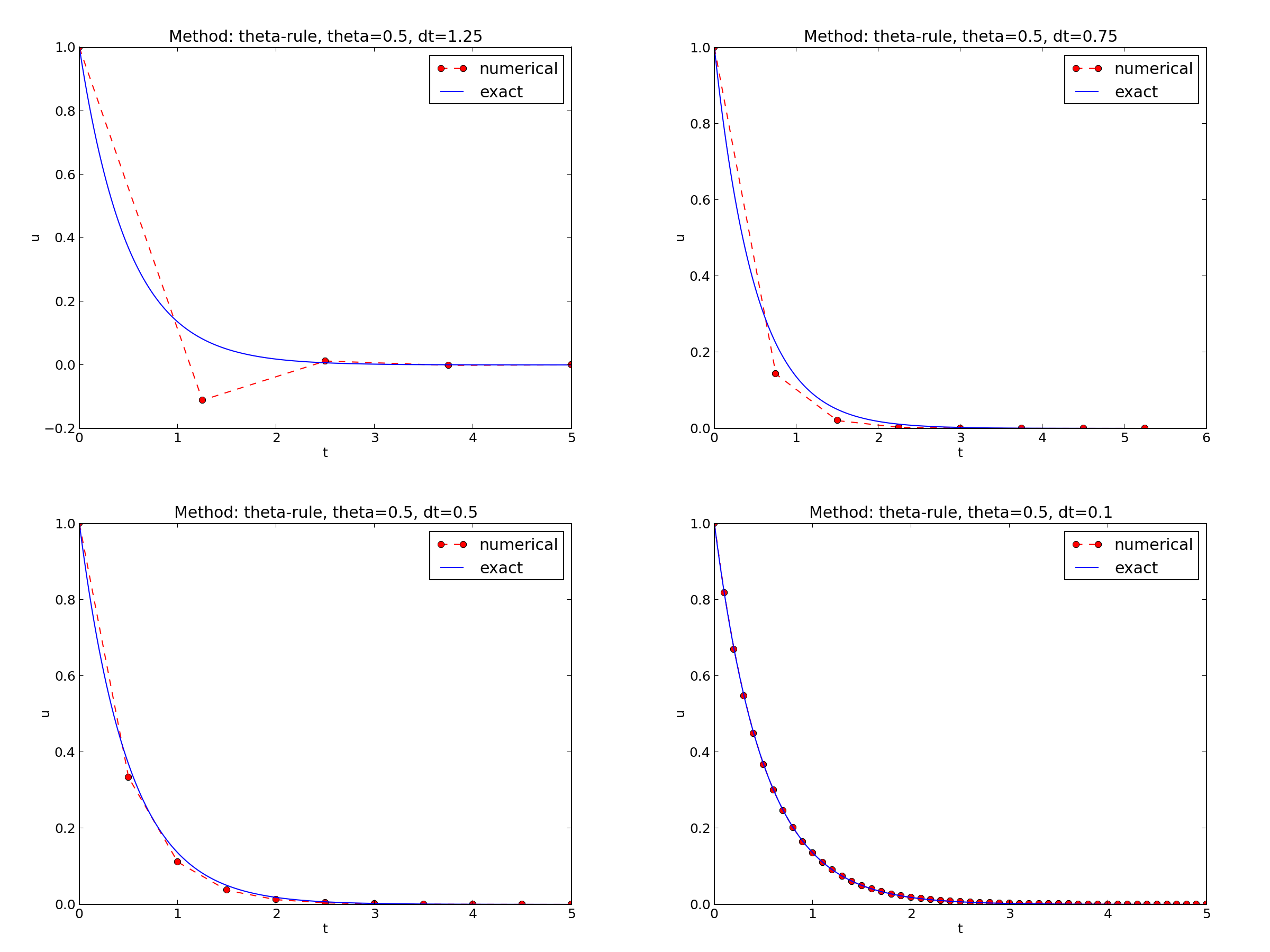
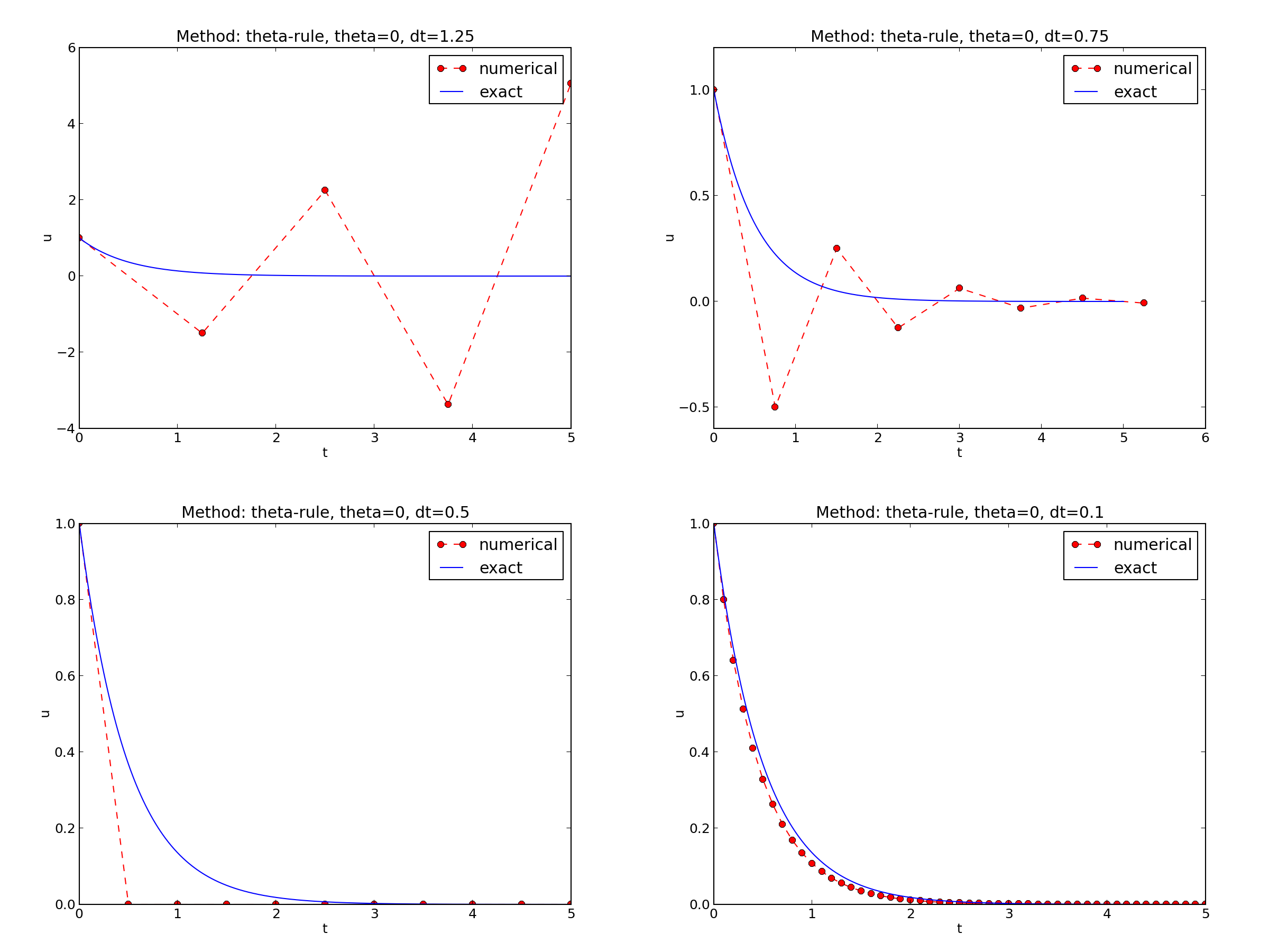
Encouraging numerical solutions
\( I=1 \), \( a=2 \), \( \theta =1,0.5, 0 \), \( \Delta t=1.25, 0.75, 0.5, 0.1 \).
Discouraging numerical solutions; Crank-Nicolson
Discouraging numerical solutions; Forward Euler
Summary of observations
The characteristics of the displayed curves can be summarized as follows:
- The Backward Euler scheme always gives a monotone solution, lying above the exact solution.
- The Crank-Nicolson scheme gives the most accurate results, but for \( \Delta t=1.25 \) the solution oscillates.
- The Forward Euler scheme gives a growing, oscillating solution for \( \Delta t=1.25 \); a decaying, oscillating solution for \( \Delta t=0.75 \); a strange solution \( u^n=0 \) for \( n\geq 1 \) when \( \Delta t=0.5 \); and a solution seemingly as accurate as the one by the Backward Euler scheme for \( \Delta t = 0.1 \), but the curve lies below the exact solution.
Problem setting
We ask the question
- Under what circumstances, i.e., values of the input data \( I \), \( a \), and \( \Delta t \) will the Forward Euler and Crank-Nicolson schemes result in undesired oscillatory solutions?
Techniques of investigation:
- Numerical experiments
- Mathematical analysis
Another question to be raised is
- How does \( \Delta t \) impact the error in the numerical solution?
Experimental investigation of oscillatory solutions
The solution is oscillatory if
$$ u^{n} > u^{n-1}$$
("Safe choices" of \( \Delta t \) lie
under the following curve as a function of \( a \).)
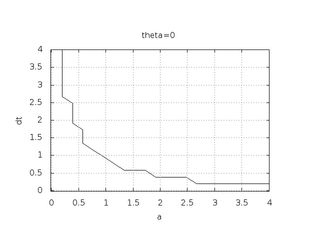
Seems that \( a\Delta t < 1 \) for FE and 2 for CN.
Exact numerical solution
Starting with \( u^0=I \), the simple recursion (2) can be applied repeatedly \( n \) times, with the result that
$$
\begin{equation}
u^{n} = IA^n,\quad A = \frac{1 - (1-\theta) a\Delta t}{1 + \theta a\Delta t}
\tag{3}
\end{equation}
$$
Such a formula for the exact discrete solution is unusual to obtain in practice, but very handy for our analysis here.
Note: An exact dicrete solution fulfills a discrete equation (without round-off errors), whereas an exact solution fulfills the original mathematical equation.
Stability
Since \( u^n=I A^n \),
- \( A < 0 \) gives a factor \( (-1)^n \) and oscillatory solutions
- \( |A|>1 \) gives growing solutions
- Recall: the exact solution is monotone and decaying
- If these qualitative properties are not met, we say that the numerical solution is unstable
Computation of stability in this problem
\( A < 0 \) if
$$
\frac{1 - (1-\theta) a\Delta t}{1 + \theta a\Delta t} < 0
$$
To avoid oscillatory solutions we must have \( A> 0 \) and
$$
\begin{equation}
\Delta t < \frac{1}{(1-\theta)a}\
\tag{4}
\end{equation}
$$
- Always fulfilled for Backward Euler
- \( \Delta t \leq 1/a \) for Forward Euler
- \( \Delta t \leq 2/a \) for Crank-Nicolson
Computation of stability in this problem
\( |A|\leq 1 \) means \( -1\leq A\leq 1 \)
$$
\begin{equation}
-1\leq\frac{1 - (1-\theta) a\Delta t}{1 + \theta a\Delta t} \leq 1
\tag{5}
\end{equation}
$$
\( -1 \) is the critical limit (because \( A\le 1 \) is always satisfied):
$$
\begin{align*}
\Delta t &\leq \frac{2}{(1-2\theta)a},\quad \mbox{when }\theta < \half
\end{align*}
$$
- Always fulfilled for Backward Euler and Crank-Nicolson
- \( \Delta t \leq 2/a \) for Forward Euler
Explanation of problems with Forward Euler
- \( a\Delta t= 2\cdot 1.25=2.5 \) and \( A=-1.5 \): oscillations and growth
- \( a\Delta t = 2\cdot 0.75=1.5 \) and \( A=-0.5 \): oscillations and decay
- \( \Delta t=0.5 \) and \( A=0 \): \( u^n=0 \) for \( n>0 \)
- Smaller \( \Delta t \): qualitatively correct solution
Explanation of problems with Crank-Nicolson
- \( \Delta t=1.25 \) and \( A=-0.25 \): oscillatory solution
- Never any growing solution
Summary of stability
- Forward Euler is conditionally stable
- \( \Delta t < 2/a \) for avoiding growth
- \( \Delta t\leq 1/a \) for avoiding oscillations
- The Crank-Nicolson is unconditionally stable wrt growth and conditionally stable wrt oscillations
- \( \Delta t < 2/a \) for avoiding oscillations
- Backward Euler is unconditionally stable
Comparing amplification factors
\( u^{n+1} \) is an amplification \( A \) of \( u^n \):
$$ u^{n+1} = Au^n,\quad A = \frac{1 - (1-\theta) a\Delta t}{1 + \theta a\Delta t} $$
The exact solution is also an amplification:
$$ u(t_{n+1}) = \Aex u(t_n), \quad \Aex = e^{-a\Delta t}$$
A possible measure of accuracy: \( \Aex - A \)
Plot of amplification factors
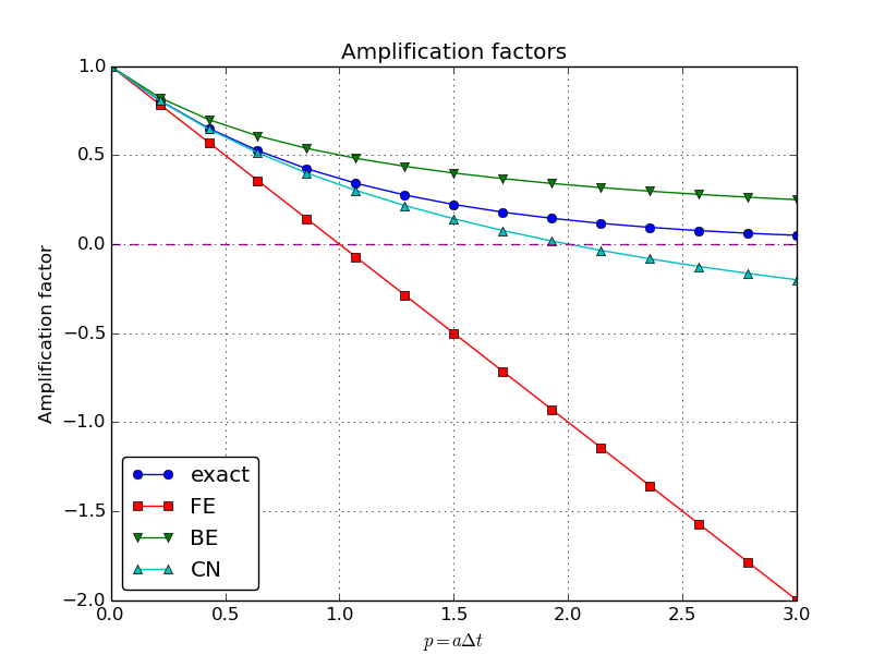
\( p=a\Delta t \) is the important parameter for numerical performance
- \( p=a\Delta t \) is a dimensionless parameter
- all expressions for stability and accuracy involve \( p \)
- Note that \( \Delta t \) alone is not so important, it is the combination with \( a \) through \( p=a\Delta t \) that matters
If we scale the model by \( \bar t=at \), \( \bar u=u/I \), we get \( d\bar u/d\bar t = -\bar u \), \( \bar u(0)=1 \) (no physical parameters!). The analysis show that \( \Delta \bar t \) is key, corresponding to \( a\Delta t \) in the unscaled model.
Series expansion of amplification factors
To investigate \( \Aex - A \) mathematically, we can Taylor expand the expression, using \( p=a\Delta t \) as variable.
>>> from sympy import *
>>> # Create p as a mathematical symbol with name 'p'
>>> p = Symbol('p')
>>> # Create a mathematical expression with p
>>> A_e = exp(-p)
>>>
>>> # Find the first 6 terms of the Taylor series of A_e
>>> A_e.series(p, 0, 6)
1 + (1/2)*p**2 - p - 1/6*p**3 - 1/120*p**5 + (1/24)*p**4 + O(p**6)

>>> theta = Symbol('theta')
>>> A = (1-(1-theta)*p)/(1+theta*p)
>>> FE = A_e.series(p, 0, 4) - A.subs(theta, 0).series(p, 0, 4)
>>> BE = A_e.series(p, 0, 4) - A.subs(theta, 1).series(p, 0, 4)
>>> half = Rational(1,2)  # exact fraction 1/2
>>> CN = A_e.series(p, 0, 4) - A.subs(theta, half).series(p, 0, 4)
>>> FE
(1/2)*p**2 - 1/6*p**3 + O(p**4)
>>> BE
-1/2*p**2 + (5/6)*p**3 + O(p**4)
>>> CN
(1/12)*p**3 + O(p**4)
Error in amplification factors
Focus: the error measure \( A-\Aex \) as function of \( \Delta t \) (recall that \( p=a\Delta t \)):
$$
\begin{equation}
A-\Aex = \left\lbrace\begin{array}{ll}
\Oof{\Delta t^2}, & \hbox{Forward and Backward Euler},\\
\Oof{\Delta t^3}, & \hbox{Crank-Nicolson}
\end{array}\right.
\tag{6}
\end{equation}
$$
The fraction of numerical and exact amplification factors
Focus: the error measure \( 1-A/\Aex \) as function of \( p=a\Delta t \):
>>> FE = 1 - (A.subs(theta, 0)/A_e).series(p, 0, 4)
>>> BE = 1 - (A.subs(theta, 1)/A_e).series(p, 0, 4)
>>> CN = 1 - (A.subs(theta, half)/A_e).series(p, 0, 4)
>>> FE
(1/2)*p**2 + (1/3)*p**3 + O(p**4)
>>> BE
-1/2*p**2 + (1/3)*p**3 + O(p**4)
>>> CN
(1/12)*p**3 + O(p**4)
Same leading-order terms as for the error measure \( A-\Aex \).
The true/global error at a point
- The error in \( A \) reflects the local (amplification) error when going from one time step to the next
- What is the global (true) error at \( t_n \)? \( e^n = \uex(t_n) - u^n = Ie^{-at_n} - IA^n \)
- Taylor series expansions of \( e^n \) simplify the expression
Computing the global error at a point
>>> n = Symbol('n')
>>> u_e = exp(-p*n)   # I=1
>>> u_n = A**n        # I=1
>>> FE = u_e.series(p, 0, 4) - u_n.subs(theta, 0).series(p, 0, 4)
>>> BE = u_e.series(p, 0, 4) - u_n.subs(theta, 1).series(p, 0, 4)
>>> CN = u_e.series(p, 0, 4) - u_n.subs(theta, half).series(p, 0, 4)
>>> FE
(1/2)*n*p**2 - 1/2*n**2*p**3 + (1/3)*n*p**3 + O(p**4)
>>> BE
(1/2)*n**2*p**3 - 1/2*n*p**2 + (1/3)*n*p**3 + O(p**4)
>>> CN
(1/12)*n*p**3 + O(p**4)
Substitute \( n \) by \( t/\Delta t \):
- Forward and Backward Euler: leading order term \( \half ta^2\Delta t \)
- Crank-Nicolson: leading order term \( \frac{1}{12}ta^3\Delta t^2 \)
Convergence
The numerical scheme is convergent if the global error \( e^n\rightarrow 0 \) as \( \Delta t\rightarrow 0 \). If the error has a leading order term \( \Delta t^r \), the convergence rate is of order \( r \).
Integrated errors
Focus: norm of the numerical error
$$ ||e^n||_{\ell^2} = \sqrt{\Delta t\sum_{n=0}^{N_t} ({\uex}(t_n) - u^n)^2}$$
Forward and Backward Euler:
$$ ||e^n||_{\ell^2} = \frac{1}{4}\sqrt{\frac{T^3}{3}} a^2\Delta t$$
Crank-Nicolson:
$$ ||e^n||_{\ell^2} = \frac{1}{12}\sqrt{\frac{T^3}{3}}a^3\Delta t^2$$
Analysis of both the pointwise and the time-integrated true errors:
- 1st order for Forward and Backward Euler
- 2nd order for Crank-Nicolson
Truncation error
- How good is the discrete equation?
- Possible answer: see how well \( \uex \) fits the discrete equation
$$ \lbrack D^{+}_t u = -au\rbrack^n$$
i.e.,
$$ \frac{u^{n+1}-u^n}{\Delta t} = -au^n$$
Insert \( \uex \) (which does not in general fulfill this discrete equation):
$$
\begin{equation}
\frac{\uex(t_{n+1})-\uex(t_n)}{\Delta t} + a\uex(t_n) = R^n \neq 0
\tag{7}
\end{equation}
$$
Computation of the truncation error
- The residual \( R^n \) is the truncation error.
- How does \( R^n \) vary with \( \Delta t \)?
Tool: Taylor expand \( \uex \) around the point where the ODE is sampled (here \( t_n \))
$$ \uex(t_{n+1}) = \uex(t_n) + \uex'(t_n)\Delta t + \half\uex''(t_n)
\Delta t^2 + \cdots $$
Inserting this Taylor series in (7) gives
$$ R^n = \uex'(t_n) + \half\uex''(t_n)\Delta t + \ldots + a\uex(t_n)$$
Now, \( \uex \) solves the ODE \( \uex'=-a\uex \), and then
$$ R^n \approx \half\uex''(t_n)\Delta t$$
This is a mathematical expression for the truncation error.
The truncation error for other schemes
Backward Euler:
$$ R^n \approx -\half\uex''(t_n)\Delta t $$
Crank-Nicolson:
$$ R^{n+\half} \approx \frac{1}{24}\uex'''(t_{n+\half})\Delta t^2$$
Consistency, stability, and convergence
- Truncation error measures the residual in the difference equations. The scheme is consistent if the truncation error goes to 0 as \( \Delta t\rightarrow 0 \). Importance: the difference equations approaches the differential equation as \( \Delta t\rightarrow 0 \).
- Stability means that the numerical solution exhibits the same qualitative properties as the exact solution. Here: monotone, decaying function.
- Convergence implies that the true (global) error \( e^n =\uex(t_n)-u^n\rightarrow 0 \) as \( \Delta t\rightarrow 0 \). This is really what we want!
The Lax equivalence theorem for linear differential equations: consistency + stability is equivalent with convergence.
(Consistency and stability is in most problems much easier to establish than convergence.)