INF5620 in a nutshell

• Numerical methods for partial differential equations (PDEs)
• How do we solve a PDE in practice and produce numbers?
• How do we trust the answer?
• Approach: simplify, understand, generalize

The new official six-point course description

After having completed INF5620 you

• can derive methods and implement them to solve frequently arising partial differential equations (PDEs) from physics and mechanics.
• have a good understanding of finite difference and finite element methods and how they are applied in linear and nonlinear PDE problems.
• can identify numerical artifacts and perform mathematical analysis to understand and cure non-physical effects.
• can apply sophisticated programming techniques in Python, combined with Cython, C, C++, and Fortran code, to create modern, flexible simulation programs.
• can construct verification tests and automate them.
• have experience with project hosting sites (GitHub), version control systems (Git), report writing (LaTeX), and Python scripting for performing reproducible computational science.

More specific contents: finite difference methods

More specific contents: finite element methods

More specific contents: nonlinear and advanced problems

Philosophy: simplify, understand, generalize

• Start with simplified ODE/PDE problems
• Learn to reason about the discretization
• Learn to implement, verify, and experiment
• Understand the method, program, and results
• Generalize the problem, method, and program

This is the power of applied mathematics!

Required software

• Our software platform: Python (sometimes combined with Cython, Fortran, C, C++)
• Important Python packages: numpy, scipy, matplotlib, sympy, fenics, scitools, ...
• Suggested installation: Run Ubuntu in a virtual machine
• Alternative: run a Vagrant machine

Assumed/ideal background

• INF1100: Python programming, solution of ODEs
• Some experience with finite difference methods
• Some analytical and numerical knowledge of PDEs
• Much experience with calculus and linear algebra
• Much experience with programming of mathematical problems
• Experience with mathematical modeling with PDEs (from physics, mechanics, geophysics, or ...)

Start-up example for the course

What if you don't have this ideal background?

• Students come to this course with very different backgrounds
• First task: summarize assumed background knowledge by going through a simple example
• Also in this example:

• Some fundamental material on software implementation and software testing
• Material on analyzing numerical methods to understand why they can fail
• Applications to real-world problems

Start-up example

Everything we do is motivated by what we need as building blocks for solving PDEs!

What to learn in the start-up example; standard topics

• How to think when constructing finite difference methods, with special focus on the Forward Euler, Backward Euler, and Crank-Nicolson (midpoint) schemes
• How to formulate a computational algorithm and translate it into Python code
• How to make curve plots of the solutions
• How to compute numerical errors
• How to compute convergence rates

What to learn in the start-up example; programming topics

• How to verify an implementation and automate verification through nose tests in Python
• How to structure code in terms of functions, classes, and modules
• How to work with Python concepts such as arrays, lists, dictionaries, lambda functions, functions in functions (closures), doctests, unit tests, command-line interfaces, graphical user interfaces
• How to perform array computing and understand the difference from scalar computing
• How to conduct and automate large-scale numerical experiments
• How to generate scientific reports

What to learn in the start-up example; mathematical analysis

• How to uncover numerical artifacts in the computed solution
• How to analyze the numerical schemes mathematically to understand why artifacts occur
• How to derive mathematical expressions for various measures of the error in numerical methods, frequently by using the sympy software for symbolic computation
• Introduce concepts such as finite difference operators, mesh (grid), mesh functions, stability, truncation error, consistency, and convergence

What to learn in the start-up example; generalizations

• Generalize the example to \( u'(t)=-a(t)u(t) + b(t) \)
• Present additional methods for the general nonlinear ODE \( u'=f(u,t) \), which is either a scalar ODE or a system of ODEs
• How to access professional packages for solving ODEs
• How our model equations like \( u'=-au \) arises in a wide range of phenomena in physics, biology, and finance

Finite difference methods

• The finite difference method is the simplest method for solving differential equations
• Fast to learn, derive, and implement
• A very useful tool to know, even if you aim at using the finite element or the finite volume method

Topics in the first intro to the finite difference method

A basic model for exponential decay

The world's simplest (?) ODE:

 
$$ \begin{equation*} u'(t) = -au(t),\quad u(0)=I,\ t\in (0,T] \end{equation*} $$

The ODE model has a range of applications in many fields

• Growth and decay of populations (cells, animals, human)
• Growth and decay of a fortune
• Radioactive decay
• Cooling/heating of an object
• Pressure variation in the atmosphere
• Vertical motion of a body in water/air
• Time-discretization of diffusion PDEs by Fourier techniques

See the text for details.

The ODE problem has a continuous and discrete version

Continuous problem

 
$$ \begin{equation} u' = -au,\ t\in (0,T], \quad u(0)=I \tag{1} \end{equation} $$

 
(varies with a continuous \( t \))

Discrete problem

Numerical methods applied to the continuous problem turns it into a discrete problem

 
$$ \begin{equation} u^{n+1} = \mbox{const} \cdot u^n, \quad n=0,1,\ldots N_t-1, \quad u^n=I \tag{2} \end{equation} $$

 
(varies with discrete mesh points \( t_n \))

The steps in the finite difference method

Solving a differential equation by a finite difference method consists of four steps:

1. discretizing the domain,
2. fulfilling the equation at discrete time points,
3. replacing derivatives by finite differences,
4. formulating a recursive algorithm.

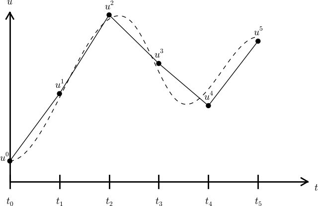
Step 1: Discretizing the domain

The time domain \( [0,T] \) is represented by a mesh: a finite number of \( N_t+1 \) points

 
$$0 = t_0 < t_1 < t_2 < \cdots < t_{N_t-1} < t_{N_t} = T$$

• We seek the solution \( u \) at the mesh points: \( u(t_n) \), \( n=1,2,\ldots,N_t \).
• Note: \( u^0 \) is known as \( I \).
• Notational short-form for the numerical approximation to \( u(t_n) \): \( u^n \)
• In the differential equation: \( u \) is the exact solution
• In the numerical method and implementation: \( u^n \) is the numerical approximation, \( \uex(t) \) is the exact solution

Step 1: Discretizing the domain

\( u^n \) is a mesh function, defined at the mesh points \( t_n \), \( n=0,\ldots,N_t \) only.

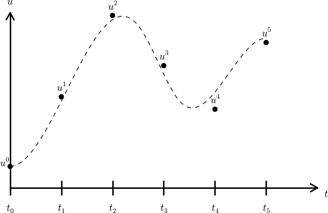
What about a mesh function between the mesh points?

Can extend the mesh function to yield values between mesh points by linear interpolation:

 
$$ \begin{equation} u(t) \approx u^n + \frac{u^{n+1}-u^n}{t_{n+1}-t_n}(t - t_n) \tag{3} \end{equation} $$

Step 2: Fulfilling the equation at discrete time points

• The ODE holds for all \( t\in (0,T] \) (infinite no of points)
• Idea: let the ODE be valid at the mesh points only (finite no of points)

 
$$ \begin{equation} u'(t_n) = -au(t_n),\quad n=1,\ldots,N_t \tag{4} \end{equation} $$

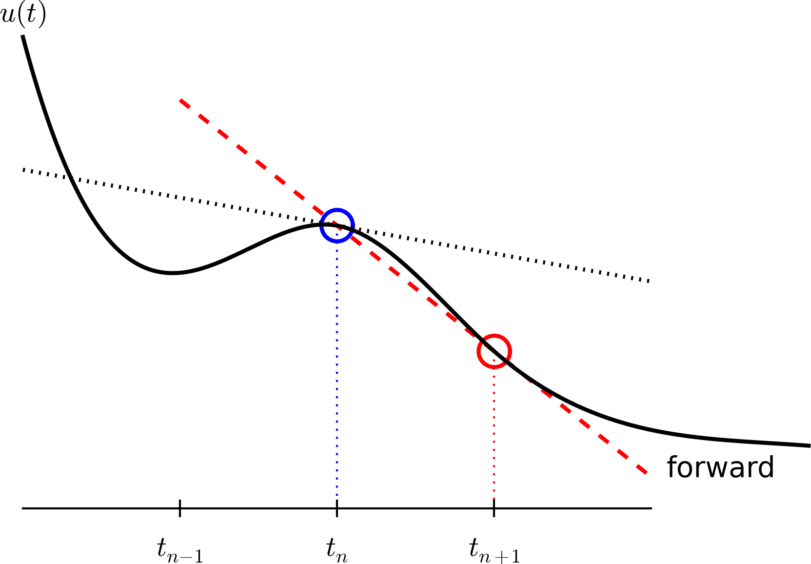
Step 3: Replacing derivatives by finite differences

Now it is time for the finite difference approximations of derivatives:

 
$$ \begin{equation} u'(t_n) \approx \frac{u^{n+1}-u^{n}}{t_{n+1}-t_n} \tag{5} \end{equation} $$

Step 3: Replacing derivatives by finite differences

Inserting the finite difference approximation in

 
$$ u'(t_n) = -au(t_n)$$

 
gives

 
$$ \begin{equation} \frac{u^{n+1}-u^{n}}{t_{n+1}-t_n} = -au^{n},\quad n=0,1,\ldots,N_t-1 \tag{6} \end{equation} $$

(Known as discrete equation, or discrete problem, or finite difference method/scheme)

Step 4: Formulating a recursive algorithm

How can we actually compute the \( u^n \) values?

• given \( u^0=I \)
• compute \( u^1 \) from \( u^0 \)
• compute \( u^2 \) from \( u^1 \)
• compute \( u^3 \) from \( u^2 \) (and so forth)

In general: we have \( u^n \) and seek \( u^{n+1} \)

Let us apply the scheme by hand

Assume constant time spacing: \( \Delta t = t_{n+1}-t_n=\mbox{const} \)

 
$$ \begin{align*} u_0 &= I,\\ u_1 & = u^0 - a\Delta t u^0 = I(1-a\Delta t),\\ u_2 & = I(1-a\Delta t)^2,\\ u^3 &= I(1-a\Delta t)^3,\\ &\vdots\\ u^{N_t} &= I(1-a\Delta t)^{N_t} \end{align*} $$

Ooops - we can find the numerical solution by hand (in this simple example)! No need for a computer (yet)...

A backward difference

Here is another finite difference approximation to the derivative (backward difference):

 
$$ \begin{equation} u'(t_n) \approx \frac{u^{n}-u^{n-1}}{t_{n}-t_{n-1}} \tag{8} \end{equation} $$

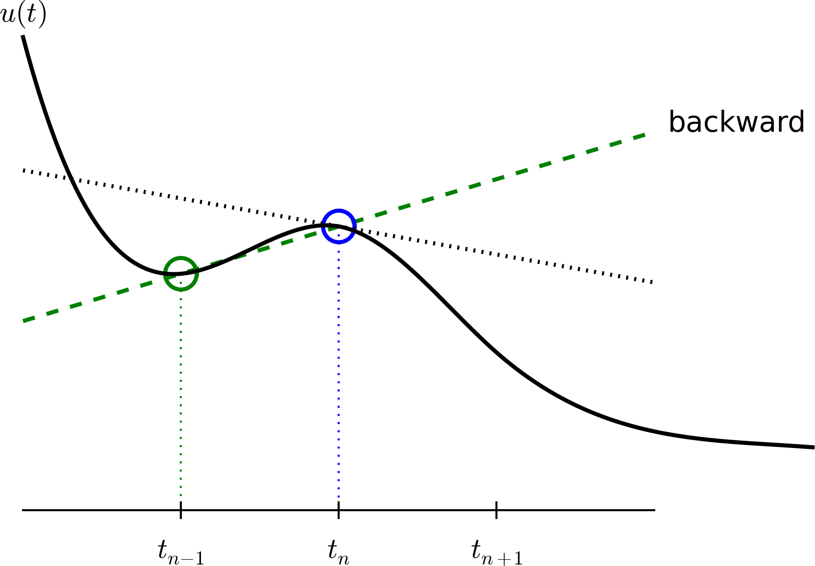
The Backward Euler scheme

Inserting the finite difference approximation in \( u'(t_n)=-au(t_n) \) yields the Backward Euler (BE) scheme:

 
$$ \begin{equation} \frac{u^{n}-u^{n-1}}{t_{n}-t_{n-1}} = -a u^n \tag{9} \end{equation} $$

 
Solve with respect to the unknown \( u^{n+1} \):

 
$$ \begin{equation} u^{n+1} = \frac{1}{1+ a(t_{n+1}-t_n)} u^n \tag{10} \end{equation} $$

A centered difference

Centered differences are better approximations than forward or backward differences.

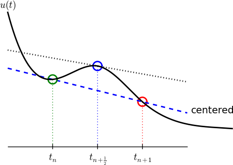
The Crank-Nicolson scheme; ideas

Idea 1: let the ODE hold at \( t_{n+\half} \)

 
$$ u'(t_{n+\half}) = -au(t_{n+\half})$$

Idea 2: approximate \( u'(t_{n+\half}) \) by a centered difference

 
$$ \begin{equation} u'(t_{n+\half}) \approx \frac{u^{n+1}-u^n}{t_{n+1}-t_n} \tag{11} \end{equation} $$

Problem: \( u(t_{n+\half}) \) is not defined, only \( u^n=u(t_n) \) and \( u^{n+1}=u(t_{n+1}) \)

Solution:

 
$$ u(t_{n+\half}) \approx \half(u^n + u^{n+1}) $$

The Crank-Nicolson scheme; result

Result:

 
$$ \begin{equation} \frac{u^{n+1}-u^n}{t_{n+1}-t_n} = -a\half (u^n + u^{n+1}) \tag{12} \end{equation} $$

Solve wrt to \( u^{n+1} \):

 
$$ \begin{equation} u^{n+1} = \frac{1-\half a(t_{n+1}-t_n)}{1 + \half a(t_{n+1}-t_n)}u^n \tag{13} \end{equation} $$

 
This is a Crank-Nicolson (CN) scheme or a midpoint or centered scheme.

The unifying \( \theta \)-rule

The Forward Euler, Backward Euler, and Crank-Nicolson schemes can be formulated as one scheme with a varying parameter \( \theta \):

 
$$ \begin{equation} \frac{u^{n+1}-u^{n}}{t_{n+1}-t_n} = -a (\theta u^{n+1} + (1-\theta) u^{n}) \tag{14} \end{equation} $$

• \( \theta =0 \): Forward Euler
• \( \theta =1 \): Backward Euler
• \( \theta =1/2 \): Crank-Nicolson
• We may alternatively choose any \( \theta\in [0,1] \).

\( u^n \) is known, solve for \( u^{n+1} \):

 
$$ \begin{equation} u^{n+1} = \frac{1 - (1-\theta) a(t_{n+1}-t_n)}{1 + \theta a(t_{n+1}-t_n)} u^n \tag{15} \end{equation} $$

Constant time step

Very common assumption (not important, but exclusively used for simplicity hereafter): constant time step \( t_{n+1}-t_n\equiv\Delta t \)

Test the understanding!

Derive Forward Euler, Backward Euler, and Crank-Nicolson schemes for Newton's law of cooling:

 
$$ T' = -k(T-T_s),\quad T(0)=T_0,\ t\in (0,t_{\mbox{end}}]$$

Physical quantities:

• \( T(t) \): temperature of an object at time \( t \)
• \( k \): parameter expressing heat loss to the surroundings
• \( T_s \): temperature of the surroundings
• \( T_0 \): initial temperature

Compact operator notation for finite differences

• Finite difference formulas can be tedious to write and read/understand
• Handy tool: finite difference operator notation
• Advantage: communicates the nature of the difference in a compact way

 
$$ \begin{equation} [D_t^- u = -au]^n \tag{20} \end{equation} $$

Specific notation for difference operators

Forward difference:

 
$$ \begin{equation} [D_t^+u]^n = \frac{u^{n+1} - u^{n}}{\Delta t} \approx \frac{d}{dt} u(t_n) \tag{21} \end{equation} $$

 
Centered difference (around \( t_n \)):

 
$$ \begin{equation} [D_tu]^n = \frac{u^{n+\half} - u^{n-\half}}{\Delta t} \approx \frac{d}{dt} u(t_n), \tag{22} \end{equation} $$

Backward difference:

 
$$ \begin{equation} [D_t^-u]^n = \frac{u^{n} - u^{n-1}}{\Delta t} \approx \frac{d}{dt} u(t_n) \tag{23} \end{equation} $$

The Backward Euler scheme with operator notation

 
$$ \begin{equation*} [D_t^-u]^n = -au^n \end{equation*} $$

Common to put the whole equation inside square brackets:

 
$$ \begin{equation} [D_t^- u = -au]^n \tag{24} \end{equation} $$

The Forward Euler scheme with operator notation

 
$$ \begin{equation} [D_t^+ u = -au]^n \tag{25} \end{equation} $$

The Crank-Nicolson scheme with operator notation

Introduce an averaging operator:

 
$$ \begin{equation} [\overline{u}^{t}]^n = \half (u^{n-\half} + u^{n+\half} ) \approx u(t_n) \tag{26} \end{equation} $$

The Crank-Nicolson scheme can then be written as

 
$$ \begin{equation} [D_t u = -a\overline{u}^t]^{n+\half} \tag{27} \end{equation} $$

Test: use the definitions and write out the above formula to see that it really is the Crank-Nicolson scheme!

Implementation

Model:

 
$$ u'(t) = -au(t),\quad t\in (0,T], \quad u(0)=I $$

Numerical method:

 
$$ u^{n+1} = \frac{1 - (1-\theta) a\Delta t}{1 + \theta a\Delta t}u^n $$

 
for \( \theta\in [0,1] \). Note

• \( \theta=0 \) gives Forward Euler
• \( \theta=1 \) gives Backward Euler
• \( \theta=1/2 \) gives Crank-Nicolson

Requirements of a program

• Compute the numerical solution \( u^n \), \( n=1,2,\ldots,N_t \)
• Display the numerical and exact solution \( \uex(t)=e^{-at} \)
• Bring evidence to a correct implementation (verification)
• Compare the numerical and the exact solution in a plot
• Compute the error \( \uex (t_n) - u^n \)
• Read its input data from the command line

Tools to learn

• Basic Python programming
• Array computing with numpy
• Plotting with matplotlib.pyplot and scitools
• File writing and reading

Why implement in Python?

• Python has a very clean, readable syntax (often known as "executable pseudo-code").
• Python code is very similar to MATLAB code (and MATLAB has a particularly widespread use for scientific computing).
• Python is a full-fledged, very powerful programming language.
• Python is similar to, but much simpler to work with and results in more reliable code than C++.

Why implement in Python?

• Python has a rich set of modules for scientific computing, and its popularity in scientific computing is rapidly growing.
• Python was made for being combined with compiled languages (C, C++, Fortran) to reuse existing numerical software and to reach high computational performance of new implementations.
• Python has extensive support for administrative task needed when doing large-scale computational investigations.
• Python has extensive support for graphics (visualization, user interfaces, web applications).
• FEniCS, a very powerful tool for solving PDEs by the finite element method, is most human-efficient to operate from Python.

Algorithm

• Store \( u^n \), \( n=0,1,\ldots,N_t \) in an array u.
• Algorithm:

  1. initialize \( u^0 \)
  2. for \( t=t_n \), \( n=1,2,\ldots,N_t \): compute \( u_n \) using the \( \theta \)-rule formula

Translation to Python function

from numpy import *

def solver(I, a, T, dt, theta):
    """Solve u'=-a*u, u(0)=I, for t in (0,T] with steps of dt."""
    Nt = int(T/dt)            # no of time intervals
    T = Nt*dt                 # adjust T to fit time step dt
    u = zeros(Nt+1)           # array of u[n] values
    t = linspace(0, T, Nt+1)  # time mesh

    u[0] = I                  # assign initial condition
    for n in range(0, Nt):    # n=0,1,...,Nt-1
        u[n+1] = (1 - (1-theta)*a*dt)/(1 + theta*dt*a)*u[n]
    return u, t

Note about the for loop: range(0, Nt, s) generates all integers from 0 to Nt in steps of s (default 1), but not including Nt (!).

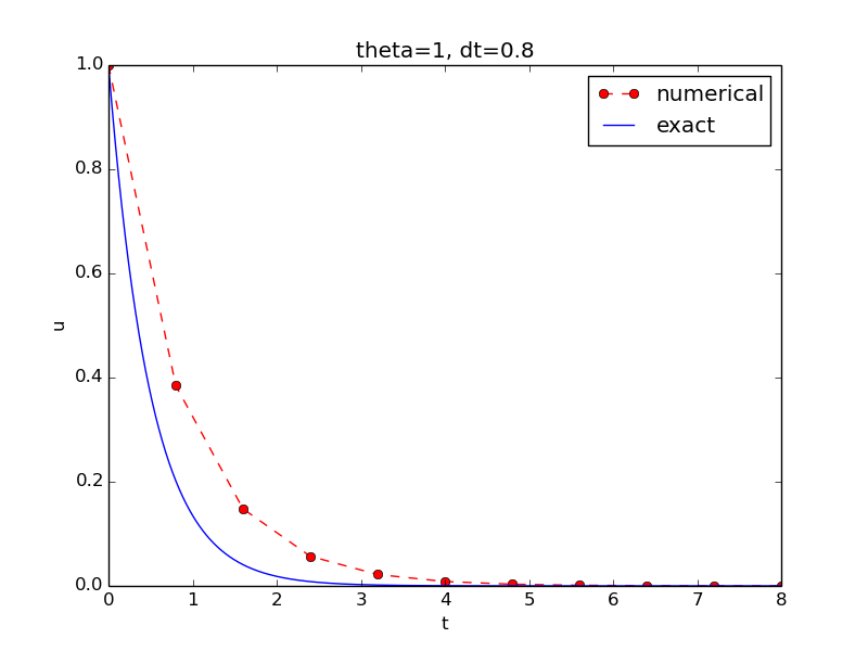
Sample call:

u, t = solver(I=1, a=2, T=8, dt=0.8, theta=1)

Integer division

Python applies integer division: 1/2 is 0, while 1./2 or 1.0/2 or 1/2. or 1/2.0 or 1.0/2.0 all give 0.5.

A safer solver function (dt = float(dt) - guarantee float):

from numpy import *

def solver(I, a, T, dt, theta):
    """Solve u'=-a*u, u(0)=I, for t in (0,T] with steps of dt."""
    dt = float(dt)            # avoid integer division
    Nt = int(round(T/dt))     # no of time intervals
    T = Nt*dt                 # adjust T to fit time step dt
    u = zeros(Nt+1)           # array of u[n] values
    t = linspace(0, T, Nt+1)  # time mesh

    u[0] = I                  # assign initial condition
    for n in range(0, Nt):    # n=0,1,...,Nt-1
        u[n+1] = (1 - (1-theta)*a*dt)/(1 + theta*dt*a)*u[n]
    return u, t

Doc strings

• First string after the function heading
• Used for documenting the function
• Automatic documentation tools can make fancy manuals for you
• Can be used for automatic testing

def solver(I, a, T, dt, theta):
    """
    Solve

        u'(t) = -a*u(t),

    with initial condition u(0)=I, for t in the time interval
    (0,T]. The time interval is divided into time steps of
    length dt.

    theta=1 corresponds to the Backward Euler scheme, theta=0
    to the Forward Euler scheme, and theta=0.5 to the Crank-
    Nicolson method.
    """
    ...

Formatting of numbers

Can control formatting of reals and integers through the printf format:

print 't=%6.3f u=%g' % (t[i], u[i])

Or the alternative format string syntax:

print 't={t:6.3f} u={u:g}'.format(t=t[i], u=u[i])

Running the program

How to run the program decay_v1.py.

Terminal> python decay_v1.py

Can also run it as "normal" Unix programs: ./decay_v1.py if the first line is

`#!/usr/bin/env python`

Then

Terminal> chmod a+rx decay_v1.py
Terminal> ./decay_v1.py

Plotting the solution

Basic syntax:

from matplotlib.pyplot import *

plot(t, u)
show()

Can (and should!) add labels on axes, title, legends.

Comparing with the exact solution

Python function for the exact solution \( \uex(t)=Ie^{-at} \):

def u_exact(t, I, a):
    return I*exp(-a*t)

Quick plotting:

u_e = u_exact(t, I, a)
plot(t, u, t, u_e)

Problem: \( \uex(t) \) applies the same mesh as \( u^n \) and looks as a piecewise linear function.

Remedy: Introduce a very fine mesh for \( \uex \).

t_e = linspace(0, T, 1001)      # fine mesh
u_e = u_exact(t_e, I, a)

plot(t_e, u_e, 'b-',            # blue line for u_e
     t,   u,   'r--o')          # red dashes w/circles

Add legends, axes labels, title, and wrap in a function

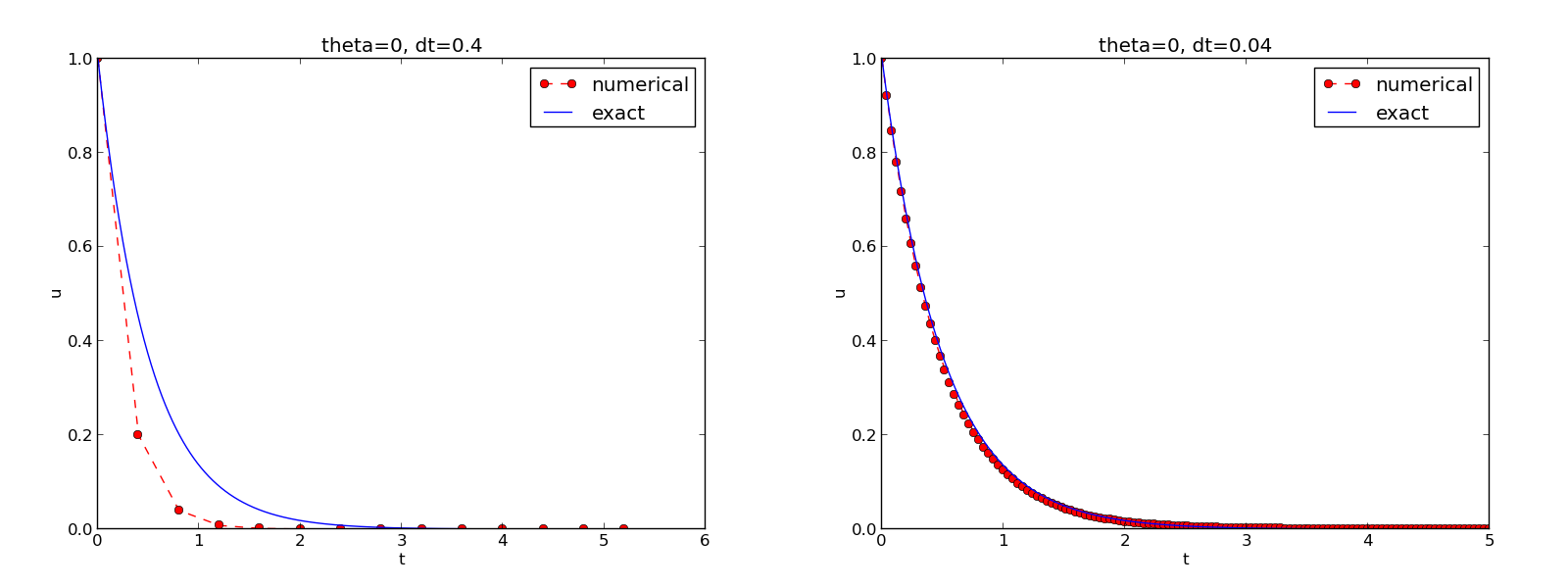
from matplotlib.pyplot import *

def plot_numerical_and_exact(theta, I, a, T, dt):
    """Compare the numerical and exact solution in a plot."""
    u, t = solver(I=I, a=a, T=T, dt=dt, theta=theta)

    t_e = linspace(0, T, 1001)        # fine mesh for u_e
    u_e = u_exact(t_e, I, a)

    plot(t,   u,   'r--o',            # red dashes w/circles
         t_e, u_e, 'b-')              # blue line for exact sol.
    legend(['numerical', 'exact'])
    xlabel('t')
    ylabel('u')
    title('theta=%g, dt=%g' % (theta, dt))
    savefig('plot_%s_%g.png' % (theta, dt))

Complete code in decay_v2.py

Plotting with SciTools

SciTools provides a unified plotting interface (Easyviz) to many different plotting packages: Matplotlib, Gnuplot, Grace, VTK, OpenDX, ...

Can use Matplotlib (MATLAB-like) syntax, or a more compact plot function syntax:

from scitools.std import *

plot(t,   u,   'r--o',           # red dashes w/circles
     t_e, u_e, 'b-',             # blue line for exact sol.
     legend=['numerical', 'exact'],
     xlabel='t',
     ylabel='u',
     title='theta=%g, dt=%g' % (theta, dt),
     savefig='%s_%g.png' % (theta2name[theta], dt),
     show=True)

Change backend (plotting engine, Matplotlib by default):

Terminal> python decay_plot_st.py --SCITOOLS_easyviz_backend gnuplot
Terminal> python decay_plot_st.py --SCITOOLS_easyviz_backend grace

Verifying the implementation

• Verification = bring evidence that the program works
• Find suitable test problems
• Make function for each test problem
• Later: put the verification tests in a professional testing framework

Simplest method: run a few algorithmic steps by hand

Use a calculator (\( I=0.1 \), \( \theta=0.8 \), \( \Delta t =0.8 \)):

 
$$ A\equiv \frac{1 - (1-\theta) a\Delta t}{1 + \theta a \Delta t} = 0.298245614035$$

 
$$ \begin{align*} u^1 &= AI=0.0298245614035,\\ u^2 &= Au^1= 0.00889504462912,\\ u^3 &=Au^2= 0.00265290804728 \end{align*} $$

See the function test_solver_three_steps in decay_v3.py.

Comparison with an exact discrete solution

Define

 
$$ A = \frac{1 - (1-\theta) a\Delta t}{1 + \theta a \Delta t}$$

 
Repeated use of the \( \theta \)-rule:

 
$$ \begin{align*} u^0 &= I,\\ u^1 &= Au^0 = AI\\ u^n &= A^nu^{n-1} = A^nI \end{align*} $$

Making a test based on an exact discrete solution

The exact discrete solution is

 
$$ \begin{equation} u^n = IA^n \tag{28} \end{equation} $$

Test if

 
$$ \max_n |u^n - \uex(t_n)| < \epsilon\sim 10^{-15}$$

Implementation in decay_verf2.py.

Test the understanding!

Make a program for solving Newton's law of cooling

 
$$ T' = -k(T-T_s),\quad T(0)=T_0,\ t\in (0,t_{\mbox{end}}]$$

 
with the Forward Euler, Backward Euler, and Crank-Nicolson schemes (or a \( \theta \) scheme). Verify the implementation.

Computing the numerical error as a mesh function

Task: compute the numerical error \( e^n = \uex(t_n) - u^n \)

Exact solution: \( \uex(t)=Ie^{-at} \), implemented as

def u_exact(t, I, a):
    return I*exp(-a*t)

Compute \( e^n \) by

u, t = solver(I, a, T, dt, theta)  # Numerical solution
u_e = u_exact(t, I, a)
e = u_e - u

Computing the norm of the error

• \( e^n \) is a mesh function
• Usually we want one number for the error
• Use a norm of \( e^n \)

Norms of a function \( f(t) \):

 
$$ \begin{align} ||f||_{L^2} &= \left( \int_0^T f(t)^2 dt\right)^{1/2} \tag{29}\\ ||f||_{L^1} &= \int_0^T |f(t)| dt \tag{30}\\ ||f||_{L^\infty} &= \max_{t\in [0,T]}|f(t)| \tag{31} \end{align} $$

Norms of mesh functions

• Problem: \( f^n =f(t_n) \) is a mesh function and hence not defined for all \( t \). How to integrate \( f^n \)?
• Idea: Apply a numerical integration rule, using only the mesh points of the mesh function.

The Trapezoidal rule:

 
$$ ||f^n|| = \left(\Delta t\left(\half(f^0)^2 + \half(f^{N_t})^2 + \sum_{n=1}^{N_t-1} (f^n)^2\right)\right)^{1/2} $$

Common simplification yields the \( L^2 \) norm of a mesh function:

 
$$ ||f^n||_{\ell^2} = \left(\Delta t\sum_{n=0}^{N_t} (f^n)^2\right)^{1/2}$$

Implementation of the norm of the error

 
$$ E = ||e^n||_{\ell^2} = \sqrt{\Delta t\sum_{n=0}^{N_t} (e^n)^2}$$

Python w/array arithmetics:

e = u_exact(t) - u
E = sqrt(dt*sum(e**2))

Comment on array vs scalar computation

Scalar computing of E = sqrt(dt*sum(e**2)):

m = len(u)     # length of u array (alt: u.size)
u_e = zeros(m)
t = 0
for i in range(m):
    u_e[i] = u_exact(t, a, I)
    t = t + dt
e = zeros(m)
for i in range(m):
    e[i] = u_e[i] - u[i]
s = 0  # summation variable
for i in range(m):
    s = s + e[i]**2
error = sqrt(dt*s)

Obviously, scalar computing

• takes more code
• is less readable
• runs much slower

Memory-saving implementation

• Note 1: we store the entire array u, i.e., \( u^n \) for \( n=0,1,\ldots,N_t \)
• Note 2: the formula for \( u^{n+1} \) needs \( u^n \) only, not \( u^{n-1} \), \( u^{n-2} \), ...
• No need to store more than \( u^{n+1} \) and \( u^{n} \)
• Extremely important when solving PDEs
• No practical importance here (much memory available)
• But let's illustrate how to do save memory!
• Idea 1: store \( u^{n+1} \) in u, \( u^n \) in u_1 (float)
• Idea 2: store u in a file, read file later for plotting

Memory-saving solver function

def solver_memsave(I, a, T, dt, theta, filename='sol.dat'):
    """
    Solve u'=-a*u, u(0)=I, for t in (0,T] with steps of dt.
    Minimum use of memory. The solution is stored in a file
    (with name filename) for later plotting.
    """
    dt = float(dt)         # avoid integer division
    Nt = int(round(T/dt))  # no of intervals

    outfile = open(filename, 'w')
    # u: time level n+1, u_1: time level n
    t = 0
    u_1 = I
    outfile.write('%.16E  %.16E\n' % (t, u_1))
    for n in range(1, Nt+1):
        u = (1 - (1-theta)*a*dt)/(1 + theta*dt*a)*u_1
        u_1 = u
        t += dt
        outfile.write('%.16E  %.16E\n' % (t, u))
    outfile.close()
    return u, t

Reading computed data from file

def read_file(filename='sol.dat'):
    infile = open(filename, 'r')
    u = [];  t = []
    for line in infile:
        words = line.split()
        if len(words) != 2:
            print 'Found more than two numbers on a line!', words
            sys.exit(1)  # abort
        t.append(float(words[0]))
        u.append(float(words[1]))
    return np.array(t), np.array(u)

Simpler code with numpy functionality for reading/writing tabular data:

def read_file_numpy(filename='sol.dat'):
    data = np.loadtxt(filename)
    t = data[:,0]
    u = data[:,1]
    return t, u

Similar function np.savetxt, but then we need all \( u^n \) and \( t^n \) values in a two-dimensional array (which we try to prevent now!).

Usage of memory-saving code

def explore(I, a, T, dt, theta=0.5, makeplot=True):
    filename = 'u.dat'
    u, t = solver_memsave(I, a, T, dt, theta, filename)

    t, u = read_file(filename)
    u_e = u_exact(t, I, a)
    e = u_e - u
    E = np.sqrt(dt*np.sum(e**2))
    if makeplot:
        plt.figure()
        ...

Complete program: decay_memsave.py.