Finite difference methods for diffusion processes

Author:Hans Petter Langtangen Date:Dec 14, 2013

Note: VERY PRELIMINARY VERSION

The 1D diffusion equation

index{diffusion equation, 1D} index{heat equation, 1D}

The famous diffusion equation, also known as the heat equation, reads

\[\frac{\partial u}{\partial t} = \alpha \frac{\partial^2 u}{\partial x^2},\]

where \(u(x,t)\) is the unknown function to be solved for, \(x\) is a coordinate in space, and \(t\) is time. The coefficient \(\alpha\) is the diffusion coefficient and determines how fast \(u\) changes in time. A quick short form for the diffusion equation is \(u_t = \alpha u_{xx}\).

Compared to the wave equation, \(u_{tt}=c^2u_{xx}\), which looks very similar, but the diffusion equation features solutions that are very different from those of the wave equation. Also, the diffusion equation makes quite different demands to the numerical methods.

Typical diffusion problems may experience rapid change in the very beginning, but then the evolution of \(u\) becomes slower and slower. The solution is usually very smooth, and after some time, one cannot recognize the initial shape of \(u\). This is in sharp contrast to solutions of the wave equation where the initial shape is preserved - the solution is basically a moving initial condition. The standard wave equation \(u_{tt}=c^2u_{xx}\) has solutions that propagates with speed \(c\) forever, without changing shape, while the diffusion equation converges to a stationary solution \(\bar u(x)\) as \(t\rightarrow\infty\). In this limit, \(u_t=0\), and \(\bar u\) is governed by \(\bar u''(x)=0\). This stationary limit of the diffusion equation is called the Laplace equation and arises in a very wide range of applications throughout the sciences.

It is possible to solve for \(u(x,t)\) using a explicit scheme, but the time step restrictions soon become much less favorable than for an explicit scheme for the wave equation. And of more importance, since the solution \(u\) of the diffusion equation is very smooth and changes slowly, small time steps are not convenient and not required by accuracy as the diffusion process converges to a stationary state.

The initial-boundary value problem for 1D diffusion

To obtain a unique solution of the diffusion equation, or equivalently, to apply numerical methods, we need initial and boundary conditions. The diffusion equation goes with one initial condition \(u(x,0)=I(x)\), where \(I\) is a prescribed function. One boundary condition is required at each point on the boundary, which in 1D means that \(u\) must be known, \(u_x\) must be known, or some combination of them.

We shall start with the simplest boundary condition: \(u=0\). The complete initial-boundary value diffusion problem in one space dimension can then be specified as

(1)\[ \frac{\partial u}{\partial t} = \alpha \frac{\partial^2 u}{\partial x^2}, \quad x\in (0,L),\ t\in (0,T]\]

(2)\[ u(x,0) = I(x), \quad x\in [0,L]\]

(3)\[\begin{split} u(0,t) = 0, \quad t>0,\end{split}\]

(4)\[\begin{split} u(L,t) = 0, \quad t>0{\thinspace .}\end{split}\]

Equation (1) is known as a one-dimensional diffusion equation, also often referred to as a heat equation. With only a first-order derivative in time, only one initial condition is needed, while the second-order derivative in space leads to a demand for two boundary conditions. The parameter \(\alpha\) must be given and is referred to as the diffusion coefficient.

Diffusion equations like (1) have a wide range of applications throughout physical, biological, and financial sciences. One of the most common applications is propagation of heat, where \(u(x,t)\) represents the temperature of some substance at point \(x\) and time \(t\). The section diffu:app goes into several widely occurring applications.

Forward Euler scheme

The first step in the discretization procedure is to replace the domain \([0,L]\times [0,T]\) by a set of mesh points. Here we apply equally spaced mesh points

\[x_i=i\Delta x,\quad i=0,\ldots,N_x,\]

and

\[t_n=n\Delta t,\quad n=0,\ldots,N_t {\thinspace .}\]

Moreover, \(u^n_i\) denotes the mesh function that approximates \(u(x_i,t_n)\) for \(i=0,\ldots,N_x\) and \(n=0,\ldots,N_t\). Requiring the PDE (1) to be fulfilled at a mesh point \((x_i,t_n)\) leads to the equation

(5)\[ \frac{\partial}{\partial t} u(x_i, t_n) = \alpha\frac{\partial^2}{\partial x^2} u(x_i, t_n),\]

The next step is to replace the derivatives by finite difference approximations. The computationally simplest method arises from using a forward difference in time and a central difference in space:

(6)\[ [D_t^+ u = \alpha D_xD_x u]^n_i {\thinspace .}\]

Written out,

(7)\[ \frac{u^{n+1}_i-u^n_i}{\Delta t} = \alpha \frac{u^{n}_{i+1} - 2u^n_i + u^n_{i-1}}{\Delta x^2} {\thinspace .}\]

We have turned the PDE into algebraic equations, also often called discrete equations. The key property of the equations is that they are algebraic, which makes them easy to solve. As usual, we anticipate that \(u^n_i\) is already computed such that \(u^{n+1}_i\) is the only unknown in (7). Solving with respect to this unknown is easy:

(8)\[ u^{n+1}_i = u^n_i + \alpha\frac{\Delta t}{\Delta x^2}\left( u^{n}_{i+1} - 2u^n_i + u^n_{i-1}\right) {\thinspace .}\]

The computational algorithm then becomes

1. compute $u^0_i=I(x_i)$for \(i=0,\ldots,N_x\)
2. for \(n=0,1,\ldots,N_t\):

1. apply (8) for all the internal spatial points \(i=1,\ldots,N_x-1\)
2. set the boundary values \(u^{n+1}_i=0\) for \(i=0\) and \(i=N_x\)

The algorithm is compactly fully specified in Python:

x = linspace(0, L, Nx+1)    # mesh points in space
dx = x[1] - x[0]
t = linspace(0, T, Nt+1)    # mesh points in time
dt = t[1] - t[0]
C = a*dt/dx**2
u   = zeros(Nx+1)
u_1 = zeros(Nx+1)

# Set initial condition u(x,0) = I(x)
for i in range(0, Nx+1):
    u_1[i] = I(x[i])

for n in range(0, Nt):
    # Compute u at inner mesh points
    for i in range(1, Nx):
        u[i] = u_1[i] + C*(u_1[i-1] - 2*u_1[i] + u_1[i+1])

    # Insert boundary conditions
    u[0] = 0;  u[Nx] = 0

    # Update u_1 before next step
    u_1[:]= u

Backward Euler Scheme

We now apply a backward difference in time in (5), but the same central difference in space:

(9)\[ [D_t^- u = D_xD_x u]^n_i,\]

which written out reads

(10)\[ \frac{u^{n}_i-u^{n-1}_i}{\Delta t} = \alpha\frac{u^{n}_{i+1} - 2u^n_i + u^n_{i-1}}{\Delta x^2} {\thinspace .}\]

Now we assume \(u^{n-1}_i\) is computed, but all quantities at the “new” time level \(n\) are unknown. This time it is not possible to solve with respect to \(u_i^{n}\) because this value couples to its neighbors in space, \(u^n_{i-1}\) and \(u^n_{i+1}\), which are also unknown. Let us examine this fact for the case when \(N_x=3\). Equation (10) written for \(i=1,\ldots,Nx-1= 1,2\) becomes

\[\frac{u^{n}_1-u^{n-1}_1}{\Delta t} = \alpha\frac{u^{n}_{2} - 2u^n_1 + u^n_{0}}{\Delta x^2}\]

\[\frac{u^{n}_2-u^{n-1}_2}{\Delta t} = \alpha\frac{u^{n}_{3} - 2u^n_2 + u^n_{1}}{\Delta x^2}\]

The boundary values \(u^n_0\) and \(u^n_3\) are known as zero. Collecting the unknown new values \(u^n_1\) and \(u^n_2\) on the left-hand side gives

\[\left(1+ 2\alpha\frac{\Delta t}{\Delta x^2}\right) u^{n}_1 - \alpha\frac{\Delta t}{\Delta x^2} u^{n}_{2} = u^{n-1}_1,\]

\[- \alpha\frac{\Delta t}{\Delta x^2} u^{n}_{1} + \left(1+ 2\alpha\frac{\Delta t}{\Delta x^2}\right) u^{n}_2 = u^{n-1}_2 {\thinspace .}\]

This is a coupled \(2\times 2\) system of algebraic equations for the unknowns \(u^n_1\) and \(u^n_2\). Discretization methods that lead to a coupled system of equations for the unknown function at a new time level are said to be implicit methods. The counterpart, explicit methods, refers to discretization methods where there is a simple explicit formula for the values of the unknown function at each of the spatial mesh points at the new time level. From an implementational point of view, implicit methods are more comprehensive to code since they require the solution of coupled equations, i.e., a matrix system, at each time level.

In the general case, (10) gives rise to a coupled \((Nx-1)\times (Nx-1)\) system of algebraic equations for all the unknown \(u^n_i\) at the interior spatial points \(i=1,\ldots,Nx-1\). Collecting the unknowns on the left-hand side, and introducing the quantity

\[C = \alpha\frac{\Delta t}{\Delta x^2},\]

(10) can be written

(11)\[ - Cu^n_{i-1} + \left(1+ 2C\right) u^{n}_i - Cu^n_{i+1} = u_{i-1}^{n-1},\]

for \(i=1,\ldots,Nx-1\). One can either view these equations as a system for where the \(u^{n}_i\) values at the internal grid points, \(i=1,\ldots,N_x-1\), are unknown, or we may append the boundary values \(u^n_0\) and \(u^n_{N_x}\) to the system. In the latter case, all \(u^n_i\) for \(i=0,\ldots,N_x\) are unknown and we must add the boundary equations to the \(N_x-1\) equations in (11):

(12)\[ u_0^n = 0,\]

(13)\[ u_{N_x}^n = 0{\thinspace .}\]

A coupled system of algebraic equations can be written on matrix form, and this is important if we want to call up ready-made software for solving the system. The equations (11) and (12)–(13) correspond to the matrix equation

\[AU = b\]

where \(U=(u^n_0,\ldots,u^n_{N_x})\), and the matrix \(A\) has the following structure:

(14)\[\begin{split} A = \left( \begin{array}{cccccccccc} A_{0,0} & A_{0,1} & 0 &\cdots & \cdots & \cdots & \cdots & \cdots & 0 \\ A_{1,0} & A_{1,1} & 0 & \ddots & & & & & \vdots \\ 0 & A_{2,1} & A_{2,2} & A_{2,3} & \ddots & & & & \vdots \\ \vdots & \ddots & & \ddots & \ddots & 0 & & & \vdots \\ \vdots & & \ddots & \ddots & \ddots & \ddots & \ddots & & \vdots \\ \vdots & & & 0 & A_{i,i-1} & A_{i,i} & A_{i,i+1} & \ddots & \vdots \\ \vdots & & & & \ddots & \ddots & \ddots &\ddots & 0 \\ \vdots & & & & &\ddots & \ddots &\ddots & A_{N_x-1,N_x} \\ 0 &\cdots & \cdots &\cdots & \cdots & \cdots & 0 & A_{N_x,N_x-1} & A_{N_x,N_x} \end{array} \right)\end{split}\]

The nonzero elements are given by

\[A_{i,i-1} = -C\]

\[A_{i,i} = 1+ 2C\]

\[A_{i,i+1} = -C\]

for the equations for internal points, \(i=1,\ldots,N_x-1\). The equations for the boundary points correspond to

\[A_{0,0} = 1,\]

\[A_{0,1} = 0,\]

\[A_{N_x,N_x-1} = 0,\]

\[A_{N_x,N_x} = 1{\thinspace .}\]

The right-hand side \(b\) is written as

\[\begin{split}b = \left(\begin{array}{c} b_0\\ b_1\\ \vdots\\ b_i\\ \vdots\\ b_{N_x} \end{array}\right)\end{split}\]

with

\[b_0 = 0,\]

\[b_i = u^{n-1}_i,\quad i=1,\ldots,N_x-1,\]

\[b_{N_x} = 0 {\thinspace .}\]

We observe that the matrix \(A\) contains quantities that do not change in time. Therefore, \(A\) can be formed once and for all before we enter the recursive formulas for the time evolution. The right-hand side \(b\), however, must be updated at each time step. This leads to the following computational algorithm, here sketched with Python code:

x = linspace(0, L, Nx+1)   # mesh points in space
dx = x[1] - x[0]
t = linspace(0, T, N+1)    # mesh points in time
u   = zeros(Nx+1)
u_1 = zeros(Nx+1)

# Data structures for the linear system
A = zeros((Nx+1, Nx+1))
b = zeros(Nx+1)

for i in range(1, Nx):
    A[i,i-1] = -C
    A[i,i+1] = -C
    A[i,i] = 1 + 2*C
A[0,0] = A[Nx,Nx] = 1

# Set initial condition u(x,0) = I(x)
for i in range(0, Nx+1):
    u_1[i] = I(x[i])

import scipy.linalg

for n in range(0, Nt):
    # Compute b and solve linear system
    for i in range(1, Nx):
        b[i] = -u_1[i]
    b[0] = b[Nx] = 0
    u[:] = scipy.linalg.solve(A, b)

    # Update u_1 before next step
    u_1[:] = u

Sparse matrix implementation

We have seen from (14) that the matrix \(A\) is tridiagonal. The code segment above used a full, dense matrix representation of \(A\), which stores a lot of values we know are zero beforehand, and worse, the solution algorithm computes with all these zeros. With \(N_x+1\) unknowns, the work by the solution algorithm is \(\frac{1}{3} (N_x+1)^3\) and the storage requirements \((N_x+1)^2\). By utilizing the fact that \(A\) is tridiagonal and employing corresponding software tools, the work and storage demands can be proportional to \(N_x\) only.

The key idea is to apply a data structure for a tridiagonal or sparse matrix. The scipy.sparse package has relevant utilities. For example, we can store the nonzero diagonals of a matrix. The package also has linear system solvers that operate on sparse matrix data structures. The code below illustrates how we can store only the main diagonal and the upper and lower diagonals.

# Representation of sparse matrix and right-hand side
main  = zeros(Nx+1)
lower = zeros(Nx-1)
upper = zeros(Nx-1)
b     = zeros(Nx+1)

# Precompute sparse matrix
main[:] = 1 + 2*C
lower[:] = -C  #1
upper[:] = -C  #1
# Insert boundary conditions
main[0] = 1
main[Nx] = 1

A = scipy.sparse.diags(
    diagonals=[main, lower, upper],
    offsets=[0, -1, 1], shape=(Nx+1, Nx+1),
    format='csr')
print A.todense()

# Set initial condition
for i in range(0,Nx+1):
    u_1[i] = I(x[i])

for n in range(0, Nt):
    b = u_1
    b[0] = b[-1] = 0.0  # boundary conditions
    u[:] = scipy.sparse.linalg.spsolve(A, b)
    u_1[:] = u

The scipy.sparse.linalg.spsolve function utilizes the sparse storage structure of A and performs in this case a very efficient Gaussian elimination solve.

The \(\theta\) rule

The \(\theta\) rule provides a family of finite difference approximations in time:

• \(\theta=0\) gives the Forward Euler scheme in time
• \(\theta=1\) gives the Backward Euler scheme in time
• \(\theta=\frac{1}{2}\) gives the Crank-Nicolson scheme in time

Applied to the 1D diffusion problem we have

\[\frac{u^{n+1}_i-u^n_i}{\Delta t} = \alpha\left( \theta \frac{u^{n+1}_{i+1} - 2u^{n+1}_i + u^{n+1}_{i-1}}{\Delta x^2} + (1-\theta) \frac{u^{n}_{i+1} - 2u^n_i + u^n_{i-1}}{\Delta x^2}\right) {\thinspace .}\]

This scheme also leads to a matrix system with entries \(1+2C\theta\) on the main diagonal of the matrix, and \(-C\theta\) on the super- and sub-diagonal. The right-hand side entry \(b_i\) is

\[b_i = u^n_{i} + C(1-\theta) \frac{u^{n}_{i+1} - 2u^n_i + u^n_{i-1}}{\Delta x^2}{\thinspace .}\]

The Laplace and Poisson equation

The Laplace equation, \(\nabla^2 u = 0\), or the Poisson equation, \(-\nabla^2 u = f\), occur in numerous applications throughout science and engineering. We can solve 1D variants of the Laplace equations with the listed software, because we can interpret \(u_{xx}=0\) as the limiting solution of \(u_t = \alpha u_{xx}\) when \(u\) reach a steady state limit where \(u_t\rightarrow 0\). Similarly, Poisson’s equation \(-u_{xx}=f\) arises from solving \(u_t = u_{xx} + f\) and letting \(t\rightarrow\) so \(u_t\rightarrow 0\).

Technically in a program, we can simulate \(t\rightarrow\infty\) by just taking one large time step, or equivalently, set \(\alpha\) to a large value. All we need is to have \(C\) large. As \(C\rightarrow\infty\), we can from the schemes see that the limiting discrete equation becomes

\[\frac{u^{n+1}_{i+1} - 2u^{n+1}_i + u^{n+1}_{i-1}}{\Delta x^2} = 0,\]

which is nothing but the discretization \([D_xD_x u]^{n+1}_i=0\) of \(u_{xx}=0\).

The Backward Euler scheme can solve the limit equation directly and hence produce a solution of the 1D Laplace equation. With the Forward Euler scheme we must do the time stepping since \(C>1/2\) is illegal and leads to instability. We may interpret this time stepping as solving the equation system from \(u_{xx}\) by iterating on a time pseudo time variable.

Extensions

These extensions are performed exactly as for a wave equation as they only affect the spatial derivatives (which are the same as in the wave equation).

• Variable coefficients
• Neumann and Robin conditions
• 2D and 3D

Future versions of this document will for completeness and independence of the wave equation document feature info on the three points. The Robin condition is new, but straightforward to handle:

\[-{\alpha}\frac{\partial u}{\partial n} = h_T(u-U_s),\quad [-{\alpha} D_x u = h_T(u-U_s)]^n_i\]

Analysis of schemes for the diffusion equation

Properties of the solution

A particular characteristic of diffusive processes, governed by an equation like

(15)\[ u_t = \alpha u_{xx},\]

is that the initial shape \(u(x,0)=I(x)\) spreads out in space with time, along with a decaying amplitude. Three different examples will illustrate the spreading of \(u\) in space and the decay in time.

Similarity solution

The diffusion equation (15) admits solutions that depend on \(\eta = (x-c)/\sqrt{4\alpha t}\) for a given value of \(c\). One particular solution is

(16)\[ u(x,t) = a\,\mbox{erf}(\eta) + b,\]

where

(17)\[ \mbox{erf}(\eta) = \frac{2}{\sqrt{\pi}}\int_0^\eta e^{-\zeta^2}d\zeta,\]

is the error function, and \(a\) and \(b\) are arbitrary constants. The error function lies in \((-1,1)\), is odd around \(\eta =0\), and goes relatively quickly to \(\pm 1\):

\[\begin{split}\lim_{\eta\rightarrow -\infty}\mbox{erf}(\eta) &=-1,\\ \lim_{\eta\rightarrow \infty}\mbox{erf}(\eta) &=1,\\ \mbox{erf}(\eta) &= -\mbox{erf}(-\eta),\\ \mbox{erf}(0) &=0,\\ \mbox{erf}(2) &=0.99532227,\\ \mbox{erf}(3) &=0.99997791 {\thinspace .}\end{split}\]

As \(t\rightarrow 0\), the error function approaches a step function centered at \(x=c\). For a diffusion problem posed on the unit interval \([0,1]\), we may choose the step at \(x=1/2\) (meaning \(c=1/2\)), \(a=-1/2\), \(b=1/2\). Then

(18)\[ u(x,t) = \frac{1}{2}\left(1 - \mbox{erf}\left(\frac{x-\frac{1}{2}}{\sqrt{4\alpha t}}\right)\right) = \frac{1}{2}\mbox{erfc}\left(\frac{x-\frac{1}{2}}{\sqrt{4\alpha t}}\right),\]

where we have introduced the complementary error function \(\mbox{erfc}(\eta) = 1-\mbox{erf}(\eta)\). The solution (18) implies the boundary conditions

(19)\[ u(0,t) = \frac{1}{2}\left(1 - \mbox{erf}\left(\frac{-1/2}{\sqrt{4\alpha t}}\right)\right),\]

(20)\[ u(1,t) = \frac{1}{2}\left(1 - \mbox{erf}\left(\frac{1/2}{\sqrt{4\alpha t}}\right)\right)\]\[ {\thinspace .}\]

For small enough \(t\), \(u(0,t)\approx 1\) and \(u(1,t)\approx 1\), but as \(t\rightarrow\infty\), \(u(x,t)\rightarrow 1/2\) on \([0,1]\).

Solution for a Gaussian pulse

The standard diffusion equation \(u_t = \alpha u_{xx}\) admits a Gaussian function as solution:

(21)\[ u(x,t) = \frac{1}{\sqrt{4\pi\alpha t}} \exp{\left({-\frac{(x-c)^2}{4\alpha t}}\right)}\]\[ {\thinspace .}\]

At \(t=0\) this is a Dirac delta function, so for computational purposes one must start to view the solution at some time \(t=t_\epsilon>0\). Replacing \(t\) by \(t_\epsilon +t\) in (21) makes it easy to operate with a (new) \(t\) that starts at \(t=0\) with an initial condition with a finite width. The important feature of (21) is that the standard deviation \(\sigma\) of a sharp initial Gaussian pulse increases in time according to \(\sigma = \sqrt{2\alpha t}\), making the pulse diffuse and flatten out.

Solution for a sine component

For example, (15) admits a solution of the form

(22)\[ u(x,t) = Qe^{-at}\sin\left( kx\right)\]\[ {\thinspace .}\]

The parameters \(Q\) and \(k\) can be freely chosen, while inserting (22) in (15) gives the constraint

\[a = -\alpha k^2 {\thinspace .}\]

A very important feature is that the initial shape \(I(x)=Q\sin kx\) undergoes a damping \(\exp{(-\alpha k^2t)}\), meaning that rapid oscillations in space, corresponding to large \(k\), are very much faster dampened than slow oscillations in space, corresponding to small \(k\). This feature leads to a smoothing of the initial condition with time.

The following examples illustrates the damping properties of (22). We consider the specific problem

\[\begin{split}u_t &= u_{xx},\quad x\in (0,1),\ t\in (0,T],\\ u(0,t) &= u(1,t) = 0,\quad t\in (0,T],\\ u(x,0) & = \sin (\pi x) + 0.1\sin(100\pi x) {\thinspace .}\end{split}\]

The initial condition has been chosen such that adding two solutions like (22) constructs an analytical solution to the problem:

(23)\[ u(x,t) = e^{-\pi^2 t}\sin (\pi x) + 0.1e^{-\pi^2 10^4 t}\sin (100\pi x)\]\[ {\thinspace .}\]

Figure Evolution of the solution of a diffusion problem: initial condition (upper left), 1/100 reduction of the small waves (upper right), 1/10 reduction of the long wave (lower left), and 1/100 reduction of the long wave (lower right) illustrates the rapid damping of rapid oscillations \(\sin (100\pi x)\) and the very much slower damping of the slowly varying \(\sin (\pi x)\) term. After about \(t=0.5\cdot10^{-4}\) the rapid oscillations do not have a visible amplitude, while we have to wait until \(t\sim 0.5\) before the amplitude of the long wave \(\sin (\pi x)\) becomes very small.

Evolution of the solution of a diffusion problem: initial condition (upper left), 1/100 reduction of the small waves (upper right), 1/10 reduction of the long wave (lower left), and 1/100 reduction of the long wave (lower right)

Analysis of discrete equations

A counterpart to (22) is the complex representation of the same function:

\[u(x,t) = Qe^{-at}e^{ikx},\]

where \(i=\sqrt{-1}\) is the imaginary unit. We can add such functions, often referred to as wave components, to make a Fourier representation of a general solution of the diffusion equation:

(24)\[ u(x,t) \approx \sum_{k\in K} b_k e^{-\alpha k^2t}e^{ikx},\]

where \(K\) is a set of an infinite number of \(k\) values needed to construct the solution. In practice, however, the series is truncated and \(K\) is a finite set of \(k\) values need build a good approximate solution. Note that (23) is a special case of (24) where \(K=\{\pi, 100\pi\}\), \(b_{\pi}=1\), and \(b_{100\pi}=0.1\).

The amplitudes \(b_k\) of the individual Fourier waves must be determined from the initial condition. At \(t=0\) we have \(u\approx\sum_kb_k\exp{(ikx)}\) and find \(K\) and \(b_k\) such that

\[I(x) \approx \sum_{k\in K} b_k e^{ikx}{\thinspace .}\]

(The relevant formulas for \(b_k\) come from Fourier analysis, or equivalently, a least-squares method for approximating \(I(x)\) in a function space with basis \(\exp{(ikx)}\).)

Much insight about the behavior of numerical methods can be obtained by investigating how a wave component \(\exp{(-\alpha k^2 t)}\exp{(ikx)}\) is treated by the numerical scheme. It appears that such wave components are also solutions of the schemes, but the damping factor \(\exp{(-\alpha k^2 t)}\) varies among the schemes. To ease the forthcoming algebra, we write the damping factor as \(A^n\). The exact amplification factor corresponding to \(A\) is \({A_{\small\mbox{e}}} = \exp{(-\alpha k^2\Delta t)}\).

Analysis of the finite difference schemes

We have seen that a general solution of the diffusion equation can be built as a linear combination of basic components

\[e^{-\alpha k^2t}e^{ikx} {\thinspace .}\]

A fundamental question is whether such components are also solutions of the finite difference schemes. This is indeed the case, but the amplitude \(\exp{(-\alpha k^2t)}\) might be modified (which also happens when solving the ODE counterpart \(u'=-\alpha u\)). We therefore look for numerical solutions of the form

(25)\[ u^n_q = A^n e^{ikq\Delta x} = A^ne^{ikx},\]

where the amplification factor \(A\) must be determined by inserting the component into an actual scheme.

Stability (1)

The exact amplification factor is \({A_{\small\mbox{e}}}=\exp{(-\alpha^2 k^2\Delta t)}\). We should therefore require \(|A| < 1\) to have a decaying numerical solution as well. If \(-1\leq A<0\), \(A^n\) will change sign from time level to time level, and we get stable, non-physical oscillations in the numerical solutions that are not present in the exact solution.

Accuracy (1)

To determine how accurately a finite difference scheme treats one wave component (25), we see that the basic deviation from the exact solution is reflected in how well \(A^n\) approximates \({A_{\small\mbox{e}}}^n\), or how well \(A\) approximates \({A_{\small\mbox{e}}}\).

Analysis of the Forward Euler scheme

The Forward Euler finite difference scheme for \(u_t = \alpha u_{xx}\) can be written as

\[[D_t^+ u = \alpha D_xD_x u]^n_q{\thinspace .}\]

Inserting a wave component (25) in the scheme demands calculating the terms

\[e^{ikq\Delta x}[D_t^+ A]^n = e^{ikq\Delta x}A^n\frac{A-1}{\Delta t},\]

and

\[A^nD_xD_x [e^{ikx}]_q = A^n\left( - e^{ikq\Delta x}\frac{4}{\Delta x^2} \sin^2\left(\frac{k\Delta x}{2}\right)\right) {\thinspace .}\]

Inserting these terms in the discrete equation and dividing by \(A^n e^{ikq\Delta x}\) leads to

\[\frac{A-1}{\Delta t} = -\alpha \frac{4}{\Delta x^2}\sin^2\left( \frac{k\Delta x}{2}\right),\]

and consequently

\[A = 1 -4C\sin^2\left( \frac{k\Delta x}{2}\right),\]

where

\[C = \frac{\alpha\Delta t}{\Delta x^2} {\thinspace .}\]

The complete numerical solution is then

\[u^n_q = \left(1 -4C\sin^2\left( \frac{k\Delta x}{2}\right)\right)^ne^{ikq\Delta x} {\thinspace .}\]

Stability (2)

We easily see that \(A\leq 1\). However, the \(A\) can be less than \(-1\), which will lead to growth of a numerical wave component. The criterion \(A\geq -1\) implies

\[4C\sin^2 (p/2)\leq 2 {\thinspace .}\]

The worst case is when \(\sin^2 (p/2)=1\), so a sufficient criterion for stability is

\[C\leq {\frac{1}{2}},\]

or expressed as a condition on \(\Delta t\):

\[\Delta t\leq \frac{\Delta x^2}{2\alpha}{\thinspace .}\]

Note that halving the spatial mesh size, \(\Delta x \rightarrow {\frac{1}{2}} \Delta x\), requires \(\Delta t\) to be reduced by a factor of \(1/4\). The method hence becomes very expensive for fine spatial meshes.

Accuracy (2)

Since \(A\) is expressed in terms of \(C\) and the parameter we now call \(p=k\Delta x/2\), we also express \({A_{\small\mbox{e}}}\) by \(C\) and \(p\):

\[{A_{\small\mbox{e}}} = \exp{(-\alpha k^2\Delta t)} = \exp{(-4Cp^2)} {\thinspace .}\]

Computing the Taylor series expansion of \(A/{A_{\small\mbox{e}}}\) in terms of \(C\) can easily be done with aid of sympy:

def A_exact(C, p):
    return exp(-4*C*p**2)

def A_FE(C, p):
    return 1 - 4*C*sin(p)**2

from sympy import *
C, p = symbols('C p')
A_err_FE = A_FE(C, p)/A_exact(C, p)
print A_err_FE.series(C, 0, 6)

The result is

\[\frac{A}{{A_{\small\mbox{e}}}} = 1 - 4 C \sin^{2}p + 2C p^{2} - 16C^{2} p^{2} \sin^{2}p + 8 C^{2} p^{4} + \cdots\]

Recalling that \(C=\alpha\Delta t/\Delta x\), \(p=k\Delta x/2\), and that \(\sin^2p\leq 1\), we realize that the dominating error terms are at most

\[1 - 4\alpha \frac{\Delta t}{\Delta x^2} + \alpha\Delta t - 4\alpha^2\Delta t^2 + \alpha^2 \Delta t^2\Delta x^2 + \cdots {\thinspace .}\]

Analysis of the Backward Euler scheme

Discretizing \(u_t = \alpha u_{xx}\) by a Backward Euler scheme,

\[[D_t^- u = \alpha D_xD_x u]^n_q,\]

and inserting a wave component (25), leads to calculations similar to those arising from the Forward Euler scheme, but since

\[e^{ikq\Delta x}[D_t^- A]^n = A^ne^{ikq\Delta x}\frac{1 - A^{-1}}{\Delta t},\]

we get

\[\frac{1-A^{-1}}{\Delta t} = -\alpha \frac{4}{\Delta x^2}\sin^2\left( \frac{k\Delta x}{2}\right),\]

and then

(26)\[ A = \left(1 + 4C\sin^2p\right)^{-1}\]\[ {\thinspace .}\]

The complete numerical solution can be written

\[u^n_q = \left(1 + 4C\sin^2 p\right)^{-n} e^{ikq\Delta x} {\thinspace .}\]

Stability (3)

We see from (26) that \(0<A<1\), which means that all numerical wave components are stable and non-oscillatory for any \(\Delta t >0\).

Analysis of the Crank-Nicolson scheme

The Crank-Nicolson scheme can be written as

\[[D_t u = \alpha D_xD_x \overline{u}^x]^{n+\frac{1}{2}}_q,\]

or

\[[D_t u]^{n+\frac{1}{2}}_q = \frac{1}{2}\alpha\left( [D_xD_x u]^{n}_q + [D_xD_x u]^{n+1}_q\right) {\thinspace .}\]

Inserting (25) in the time derivative approximation leads to

\[[D_t A^n e^{ikq\Delta x}]^{n+\frac{1}{2}} = A^{n+\frac{1}{2}} e^{ikq\Delta x}\frac{A^{\frac{1}{2}}-A^{-\frac{1}{2}}}{\Delta t} = A^ne^{ikq\Delta x}\frac{A-1}{\Delta t} {\thinspace .}\]

Inserting (25) in the other terms and dividing by \(A^ne^{ikq\Delta x}\) gives the relation

\[\frac{A-1}{\Delta t} = -\frac{1}{2}\alpha\frac{4}{\Delta x^2} \sin^2\left(\frac{k\Delta x}{2}\right) (1 + A),\]

and after some more algebra,

\[A = \frac{ 1 - 2C\sin^2p}{1 + 2C\sin^2p} {\thinspace .}\]

The exact numerical solution is hence

\[u^n_q = \left(\frac{ 1 - 2C\sin^2p}{1 + 2C\sin^2p}\right)^ne^{ikp\Delta x} {\thinspace .}\]

Stability (4)

The criteria \(A>-1\) and \(A<1\) are fulfilled for any \(\Delta t >0\).

Summary of accuracy of amplification factors

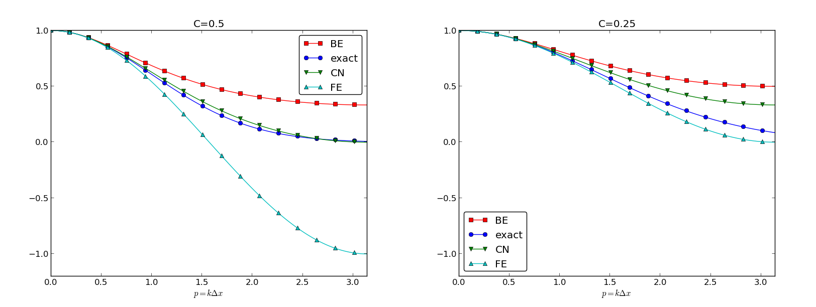
We can plot the various amplification factors against \(p=k\Delta x/2\) for different choices of the \(C\) parameter. Figures Amplification factors for large time steps, Amplification factors for time steps around the Forward Euler stability limit, and Amplification factors for small time steps show how long and small waves are damped by the various schemes compared to the exact damping. As long as all schemes are stable, the amplification factor is positive, except for Crank-Nicolson when \(C>0.5\).

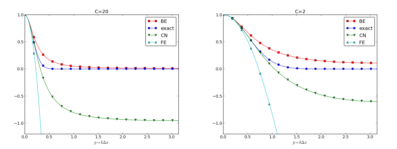
Amplification factors for large time steps

Amplification factors for time steps around the Forward Euler stability limit

Amplification factors for small time steps

The effect of negative amplification factors is that \(A^n\) changes sign from one time level to the next, thereby giving rise to oscillations in time in an animation of the solution. We see from Figure Amplification factors for large time steps that for \(C=20\), waves with \(p\geq \pi/2\) undergo a damping close to \(-1\), which means that the amplitude does not decay and that the wave component jumps up and down in time. For \(C=2\) we have a damping of a factor of 0.5 from one time level to the next, which is very much smaller than the exact damping. Short waves will therefore fail to be effectively dampened. These waves will manifest themselves as high frequency oscillatory noise in the solution.

A value \(p=\pi/4\) corresponds to four mesh points per wave length of \(e^{ikx}\), while \(p=\pi/2\) implies only two points per wave length, which is the smallest number of points we can have to represent the wave on the mesh.

To demonstrate the oscillatory behavior of the Crank-Nicolson scheme, we choose an initial condition that leads to short waves with significant amplitude. A discontinuous \(I(x)\) will in particular serve this purpose.

Run \(C=...\)...

Exercise 1: Use an analytical solution to formulate a 1D test

This exercise explores the exact solution (21). We shall formulate a diffusion problem in half of the domain for half of the Gaussian pulse. Then we shall investigate the impact of using an incorrect boundary condition, which we in general cases often are forced due if the solution needs to pass through finite boundaries undisturbed.

a) The solution (21) is seen to be symmetric at \(x=c\), because \(\partial u/\partial x =0\) always vanishes for \(x=c\). Use this property to formulate a complete initial boundary value problem in 1D involving the diffusion equation \(u_t=\alpha u_{xx}\) on \([0,L]\) with \(u_x(0,t)=0\) and \(u(L,t)\) known.

b) Use the exact solution to set up a convergence rate test for an implementation of the problem. Investigate if a one-sided difference for \(u_x(0,t)\), say \(u_0=u_1\), destroys the second-order accuracy in space.

c) Imagine that we want to solve the problem numerically on \([0,L]\), but we do not know the exact solution and cannot of that reason assign a correct Dirichlet condition at \(x=L\). One idea is to simply set \(u(L,t)=0\) since this will be an accurate approximation before the diffused pulse reaches \(x=L\) and even thereafter it might be a satisfactory condition. Let \({u_{\small\mbox{e}}}\) be the exact solution and let \(u\) be the solution of \(u_t=\alpha u_{xx}\) with an initial Gaussian pulse and the boundary conditions \(u_x(0,t)=u(L,t)=0\). Derive a diffusion problem for the error \(e={u_{\small\mbox{e}}} - u\). Solve this problem numerically using an exact Dirichlet condition at \(x=L\). Animate the evolution of the error and make a curve plot of the error measure

\[E(t)=\sqrt{\frac{\int_0^L e^2dx}{\int_0^L udx}}{\thinspace .}\]

Is this a suitable error measure for the present problem?

d) Instead of using \(u(L,t)=0\) as approximate boundary condition for letting the diffused Gaussian pulse out of our finite domain, one may try \(u_x(L,t)=0\) since the solution for large \(t\) is quite flat. Argue that this condition gives a completely wrong asymptotic solution as \(t\rightarrow 0\). To do this, integrate the diffusion equation from \(0\) to \(L\), integrate \(u_{xx}\) by parts (or use Gauss’ divergence theorem in 1D) to arrive at the important property

\[\frac{d}{dt}\int_{0}^L u(x,t)dx = 0,\]

implying that \(\int_0^Ludx\) must be constant in time, and therefore

\[\int_{0}^L u(x,t)dx = \int_{0}^LI(x)dx{\thinspace .}\]

The integral of the initial pulse is 1.

e) Another idea for an artificial boundary condition at \(x=L\) is to use a cooling law

(27)\[ -\alpha u_x = q(u - u_S),\]

where \(q\) is an unknown heat transfer coefficient and \(u_S\) is the surrounding temperature in the medium outside of \([0,L]\). (Note that arguing that \(u_S\) is approximately \(u(L,t)\) gives the \(u_x=0\) condition from the previous subexercise that is qualitatively wrong for large \(t\).) Develop a diffusion problem for the error in the solution using (27) as boundary condition. Assume one can take \(u_S=0\) “outside the domain” as \(u\rightarrow 0\) for \(x\rightarrow\infty\). Find a function \(q=q(t)\) such that the exact solution obeys the condition (27). Test some constant values of \(q\) and animate how the corresponding error function behaves. Also compute \(E(t)\) curves as suggested in subexercise b).

Filename: diffu_symmetric_gaussian.py.

Exercise 2: Use an analytical solution to formulate a 2D test

Generalize (21) to multi dimensions by assuming that one-dimensional solutions can be multiplied to solve \(u_t = \alpha\nabla^2 u\). Use this solution to formulate a 2D test case where the peak of the Gaussian is at the origin and where the domain is a rectangule in the first quadrant. Use symmetry boundary conditions \(\partial u/\partial n=0\) whereever possible, and use exact Dirichlet conditions on the remaining boundaries. Filename: diffu_symmetric_gaussian_2D.pdf.