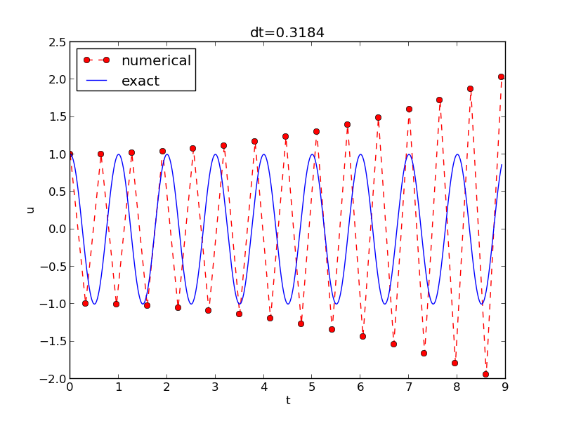
Effect of the time step on long simulations

- The numerical solution seems to have right amplitude.
- There is a phase error (reduced by reducing the time step).
- The total phase error seems to grow with time.
$$
\begin{equation}
u''t + \omega^2u = 0,\quad u(0)=I,\ u'(0)=0,\ t\in (0,T]
\tp
\tag{1}
\end{equation}
$$
Exact solution:
$$
\begin{equation}
u(t) = I\cos (\omega t)
\tp
\tag{2}
\end{equation}
$$
\( u(t) \) oscillates with constant amplitude \( I \) and
(angular) frequency \( \omega \).
Period: \( P=2\pi/\omega \).
$$
\begin{equation}
u''(t_n) + \omega^2u(t_n) = 0,\quad n=1,\ldots,N_t
\tp
\tag{3}
\end{equation}
$$
Step 3: Approximate derivative(s) by finite difference approximation(s). Very common (standard!) formula for \( u'' \):
$$
\begin{equation}
u''(t_n) \approx \frac{u^{n+1}-2u^n + u^{n-1}}{\Delta t^2}
\tp
\tag{4}
\end{equation}
$$
Use this discrete initial condition together with the ODE at \( t=0 \) to eliminate \( u^{-1} \) (insert (4) in (3)):
$$
\begin{equation}
\frac{u^{n+1}-2u^n + u^{n-1}}{\Delta t^2} = -\omega^2 u^n
\tp
\tag{5}
\end{equation}
$$
Step 4: Formulate the computational algorithm. Assume \( u^{n-1} \) and \( u^n \) are known, solve for unknown \( u^{n+1} \):
$$
\begin{equation}
u^{n+1} = 2u^n - u^{n-1} - \Delta t^2\omega^2 u^n
\tp
\tag{6}
\end{equation}
$$
Nick names for this scheme: Stormer's method or Verlet integration.
Discretize \( u'(0)=0 \) by a centered difference
$$
\begin{equation}
\frac{u^1-u^{-1}}{2\Delta t} = 0\quad\Rightarrow\quad u^{-1} = u^1
\tp
\end{equation}
$$
Inserted in (6) for \( n=0 \) gives
$$
\begin{equation}
u^1 = u^0 - \half \Delta t^2 \omega^2 u^0
\tp
\tag{7}
\end{equation}
$$
More precisly expressed in Python:
t = linspace(0, T, Nt+1)  # mesh points in time
dt = t[1] - t[0]          # constant time step.
u = zeros(Nt+1)           # solution

u[0] = I
u[1] = u[0] - 0.5*dt**2*w**2*u[0]
for n in range(1, Nt):
    u[n+1] = 2*u[n] - u[n-1] - dt**2*w**2*u[n]
Note: w is consistently used for \( \omega \) in my code.
With \( [D_tD_t u]^n \) as the finite difference approximation to \( u''(t_n) \) we can write
$$
\begin{equation}
[D_tD_t u + \omega^2 u = 0]^n
\tp
\tag{8}
\end{equation}
$$
\( [D_tD_t u]^n \) means applying a central difference with step \( \Delta t/2 \) twice:
$$ [D_t(D_t u)]^n = \frac{[D_t u]^{n+\half} - [D_t u]^{n-\half}}{\Delta t}$$
which is written out as
$$
\frac{1}{\Delta t}\left(\frac{u^{n+1}-u^n}{\Delta t} - \frac{u^{n}-u^{n-1}}{\Delta t}\right) = \frac{u^{n+1}-2u^n + u^{n-1}}{\Delta t^2}
\tp
$$
$$
\begin{equation}
[u = I]^0,\quad [D_{2t} u = 0]^0,
\end{equation}
$$
where \( [D_{2t} u]^n \) is defined as
$$
\begin{equation}
[D_{2t} u]^n = \frac{u^{n+1} - u^{n-1}}{2\Delta t}
\tp
\end{equation}
$$
\( u \) is often displacement/position, \( u' \) is velocity and can be computed by
$$
\begin{equation}
u'(t_n) \approx \frac{u^{n+1}-u^{n-1}}{2\Delta t} = [D_{2t}u]^n
\tp
\end{equation}
$$
from numpy import *
from matplotlib.pyplot import *
from vib_empirical_analysis import minmax, periods, amplitudes

def solver(I, w, dt, T):
    """
    Solve u'' + w**2*u = 0 for t in (0,T], u(0)=I and u'(0)=0,
    by a central finite difference method with time step dt.
    """
    dt = float(dt)
    Nt = int(round(T/dt))
    u = zeros(Nt+1)
    t = linspace(0, Nt*dt, Nt+1)

    u[0] = I
    u[1] = u[0] - 0.5*dt**2*w**2*u[0]
    for n in range(1, Nt):
        u[n+1] = 2*u[n] - u[n-1] - dt**2*w**2*u[n]
    return u, t
def exact_solution(t, I, w):
    return I*cos(w*t)

def visualize(u, t, I, w):
    plot(t, u, 'r--o')
    t_fine = linspace(0, t[-1], 1001)  # very fine mesh for u_e
    u_e = exact_solution(t_fine, I, w)
    hold('on')
    plot(t_fine, u_e, 'b-')
    legend(['numerical', 'exact'], loc='upper left')
    xlabel('t')
    ylabel('u')
    dt = t[1] - t[0]
    title('dt=%g' % dt)
    umin = 1.2*u.min();  umax = -umin
    axis([t[0], t[-1], umin, umax])
    savefig('vib1.png')
    savefig('vib1.pdf')
    savefig('vib1.eps')
I = 1
w = 2*pi
dt = 0.05
num_periods = 5
P = 2*pi/w    #  one period
T = P*num_periods
u, t = solver(I, w, dt, T)
visualize(u, t, I, w, dt)
import argparse
parser = argparse.ArgumentParser()
parser.add_argument('--I', type=float, default=1.0)
parser.add_argument('--w', type=float, default=2*pi)
parser.add_argument('--dt', type=float, default=0.05)
parser.add_argument('--num_periods', type=int, default=5)
a = parser.parse_args()
I, w, dt, num_periods = a.I, a.w, a.dt, a.num_periods
Terminal> python vib_undamped.py --dt 0.05 --num_periods 40
Generates frames tmp_vib%04d.png in files. Can make movie:
Terminal> avconv -r 12 -i tmp_vib%04d.png -vcodec flv movie.flv
Can use ffmpeg instead of avconv.
| Format | Codec and filename |
| Flash | -vcodec flv movie.flv |
| MP4 | -vcodec libx64 movie.mp4 |
| Webm | -vcodec libvpx movie.webm |
| Ogg | -vcodec libtheora movie.ogg |
The next function estimates convergence rates, i.e., it
def convergence_rates(m, num_periods=8):
    """
    Return m-1 empirical estimates of the convergence rate
    based on m simulations, where the time step is halved
    for each simulation.
    """
    w = 0.35; I = 0.3
    dt = 2*pi/w/30  # 30 time step per period 2*pi/w
    T = 2*pi/w*num_periods
    dt_values = []
    E_values = []
    for i in range(m):
        u, t = solver(I, w, dt, T)
        u_e = exact_solution(t, I, w)
        E = sqrt(dt*sum((u_e-u)**2))
        dt_values.append(dt)
        E_values.append(E)
        dt = dt/2

    r = [log(E_values[i-1]/E_values[i])/
         log(dt_values[i-1]/dt_values[i])
         for i in range(1, m, 1)]
    return r
Result: r contains values equal to 2.00 - as expected!
Use final r[-1] in a unit test:
def test_convergence_rates():
    r = convergence_rates(m=5, num_periods=8)
    # Accept rate to 1 decimal place
    nt.assert_almost_equal(r[-1], 2.0, places=1)
Complete code in vib_undamped.py.
scitools.MovingPlotWindow.scitools.avplotter (ASCII vertical plotter).Example:
Terminal> python vib_undamped.py --dt 0.05 --num_periods 40
Movie of the moving plot window.
$$
u^n = IA^n = I\exp{(\tilde\omega \Delta t\, n)}=I\exp{(\tilde\omega t)} =
I\cos (\tilde\omega t) + iI\sin(\tilde \omega t)
\tp
$$
$$
\begin{align*}
[D_tD_t u]^n &= \frac{u^{n+1} - 2u^n + u^{n-1}}{\Delta t^2}\\
&= I\frac{A^{n+1} - 2A^n + A^{n-1}}{\Delta t^2}\\
&= I\frac{\exp{(i\tilde\omega(t+\Delta t))} - 2\exp{(i\tilde\omega t)} + \exp{(i\tilde\omega(t-\Delta t))}}{\Delta t^2}\\
&= I\exp{(i\tilde\omega t)}\frac{1}{\Delta t^2}\left(\exp{(i\tilde\omega(\Delta t))} + \exp{(i\tilde\omega(-\Delta t))} - 2\right)\\
&= I\exp{(i\tilde\omega t)}\frac{2}{\Delta t^2}\left(\cosh(i\tilde\omega\Delta t) -1 \right)\\
&= I\exp{(i\tilde\omega t)}\frac{2}{\Delta t^2}\left(\cos(\tilde\omega\Delta t) -1 \right)\\
&= -I\exp{(i\tilde\omega t)}\frac{4}{\Delta t^2}\sin^2(\frac{\tilde\omega\Delta t}{2})
\end{align*}
$$
The scheme (6) with \( u^n=I\exp{(i\omega\tilde\Delta t\, n)} \) inserted gives
$$
\begin{equation}
-I\exp{(i\tilde\omega t)}\frac{4}{\Delta t^2}\sin^2(\frac{\tilde\omega\Delta t}{2})
+ \omega^2 I\exp{(i\tilde\omega t)} = 0,
\end{equation}
$$
which after dividing by \( Io\exp{(i\tilde\omega t)} \) results in
$$
\begin{equation}
\frac{4}{\Delta t^2}\sin^2(\frac{\tilde\omega\Delta t}{2}) = \omega^2
\tp
\end{equation}
$$
Solve for \( \tilde\omega \):
$$
\begin{equation}
\tilde\omega = \pm \frac{2}{\Delta t}\sin^{-1}\left(\frac{\omega\Delta t}{2}\right)
\tp
\tag{9}
\end{equation}
$$
Taylor series expansion for small \( \Delta t \) gives a formula that is easier to understand:
>>> from sympy import *
>>> dt, w = symbols('dt w')
>>> w_tilde = asin(w*dt/2).series(dt, 0, 4)*2/dt
>>> print w_tilde
(dt*w + dt**3*w**3/24 + O(dt**4))/dt  # observe final /dt
$$
\begin{equation}
\tilde\omega = \omega\left( 1 + \frac{1}{24}\omega^2\Delta t^2\right) + {\cal O}(\Delta t^3)
\tp
\tag{10}
\end{equation}
$$
The numerical frequency is too large (to fast oscillations).

Recommendation: 25-30 points per period.
$$
\begin{equation}
u^n = I\cos\left(\tilde\omega n\Delta t\right),\quad
\tilde\omega = \frac{2}{\Delta t}\sin^{-1}\left(\frac{\omega\Delta t}{2}\right)
\tp
\tag{11}
\end{equation}
$$
The error mesh function,
$$ e^n = \uex(t_n) - u^n =
I\cos\left(\omega n\Delta t\right)
- I\cos\left(\tilde\omega n\Delta t\right)
$$
is ideal for verification and analysis.
Can easily show convergence:
$$ e^n\rightarrow 0 \hbox{ as }\Delta t\rightarrow 0,$$
because
$$
\lim_{\Delta t\rightarrow 0}
\tilde\omega = \lim_{\Delta t\rightarrow 0}
\frac{2}{\Delta t}\sin^{-1}\left(\frac{\omega\Delta t}{2}\right)
= \omega,
$$
by L'Hopital's rule or simply asking
(2/x)*asin(w*x/2) as x->0 in WolframAlpha.
Observations:
What is the consequence of complex \( \tilde\omega \)?
Cannot tolerate growth and must therefore demand a stability criterion
$$
\begin{equation}
\frac{\omega\Delta t}{2} \leq 1\quad\Rightarrow\quad
\Delta t \leq \frac{2}{\omega}
\tp
\end{equation}
$$
Try \( \Delta t = \frac{2}{\omega} + 9.01\cdot 10^{-5} \) (slightly too big!):
We can draw three important conclusions:
The vast collection of ODE solvers (e.g., in Odespy) cannot be applied to
$$ u'' + \omega^2 u = 0$$
unless we write this higher-order ODE as a system of 1st-order ODEs.
Introduce an auxiliary variable \( v=u' \):
$$
\begin{align}
u' &= v,
\tag{12}\\
v' &= -\omega^2 u
\tag{13}
\tp
\end{align}
$$
Initial conditions: \( u(0)=I \) and \( v(0)=0 \).
We apply the Forward Euler scheme to each component equation:
$$ [D_t^+ u = v]^n,$$
$$ [D_t^+ v = -\omega^2 u]^n,$$
or written out,
$$
\begin{align}
u^{n+1} &= u^n + \Delta t v^n,\\
v^{n+1} &= v^n -\Delta t \omega^2 u^n
\tp
\end{align}
$$
We apply the Backward Euler scheme to each component equation:
$$ [D_t^- u = v]^{n+1},$$
$$ [D_t^- v = -\omega u]^{n+1} \tp $$
Written out:
$$
\begin{align}
u^{n+1} - \Delta t v^{n+1} = u^{n},\\
v^{n+1} + \Delta t \omega^2 u^{n+1} = v^{n}
\tp
\end{align}
$$
This is a coupled \( 2\times 2 \) system for the new values at \( t=t_{n+1} \)!
$$
[D_t u = \overline{v}^t]^{n+\half},$$
$$
[D_t v = -\omega \overline{u}^t]^{n+\half}$$
The result is also a coupled system:
$$
\begin{align}
u^{n+1} - \half\Delta t v^{n+1} &= u^{n} + \half\Delta t v^{n},\\
v^{n+1} + \half\Delta t \omega^2 u^{n+1} &= v^{n}
- \half\Delta t \omega^2 u^{n}
\tp
\end{align}
$$
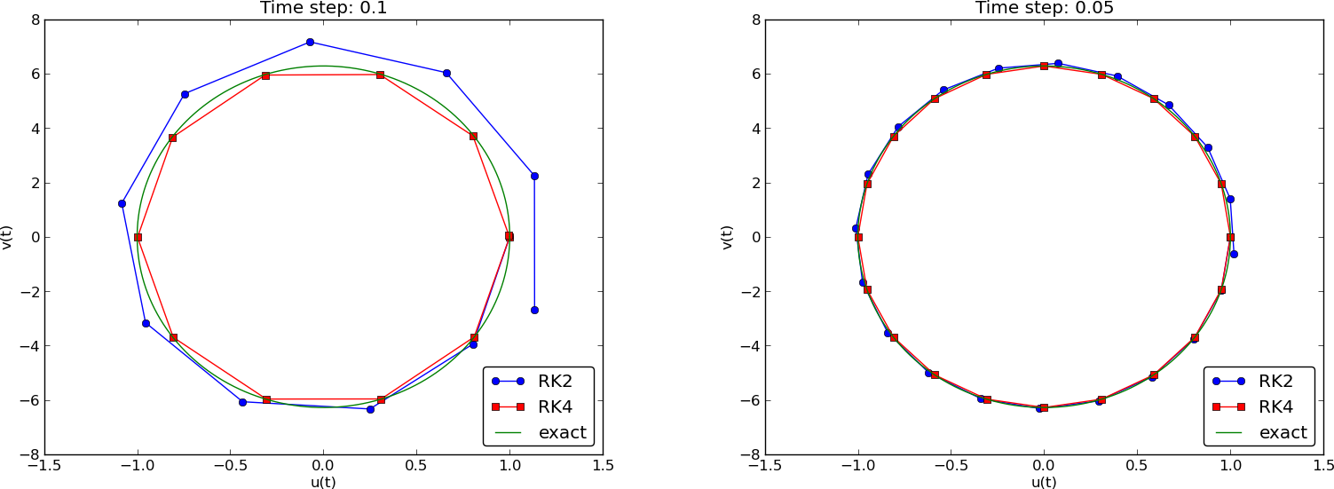
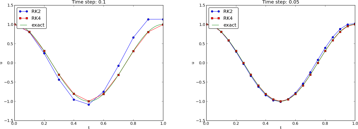
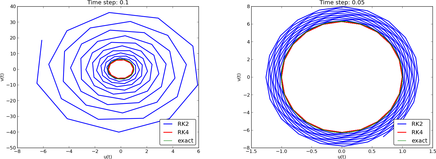
Can use Odespy to compare many methods for first-order schemes:
import odespy
import numpy as np

def f(u, t, w=1):
    u, v = u  # u is array of length 2 holding our [u, v]
    return [v, -w**2*u]

def run_solvers_and_plot(solvers, timesteps_per_period=20,
                         num_periods=1, I=1, w=2*np.pi):
    P = 2*np.pi/w  # duration of one period
    dt = P/timesteps_per_period
    Nt = num_periods*timesteps_per_period
    T = Nt*dt
    t_mesh = np.linspace(0, T, Nt+1)

    legends = []
    for solver in solvers:
        solver.set(f_kwargs={'w': w})
        solver.set_initial_condition([I, 0])
        u, t = solver.solve(t_mesh)
solvers = [
    odespy.ForwardEuler(f),
    # Implicit methods must use Newton solver to converge
    odespy.BackwardEuler(f, nonlinear_solver='Newton'),
    odespy.CrankNicolson(f, nonlinear_solver='Newton'),
    ]
Two plot types:

Note: CrankNicolson in Odespy leads to the name MidpointImplicit in plots.


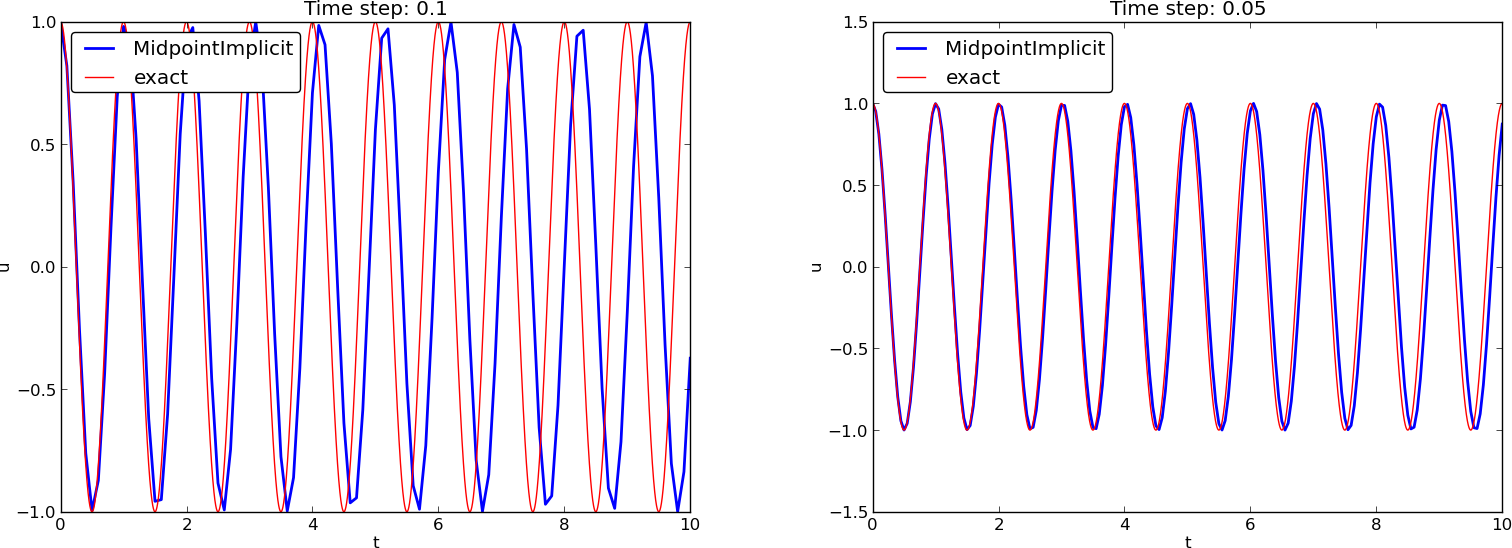
(MidpointImplicit means CrankNicolson in Odespy)
The model
$$ u'' + \omega^2 u = 0,\quad u(0)=I,\ u'(0)=V,$$
has the nice energy conservation property that
$$ E(t) = \half(u')^2 + \half\omega^2u^2 = \hbox{const}\tp$$
This can be used to check solutions.
Multiply \( u''+\omega^2u=0 \) by \( u' \) and integrate:
$$ \int_0^T u''u' dt + \int_0^T\omega^2 u u' dt = 0\tp$$
Observing that
$$ u''u' = \frac{d}{dt}\half(u')^2,\quad uu' = \frac{d}{dt} {\half}u^2,$$
we get
$$
\int_0^T (\frac{d}{dt}\half(u')^2 + \frac{d}{dt} \half\omega^2u^2)dt = E(T) - E(0),
$$
where
$$
\begin{equation}
E(t) = \half(u')^2 + \half\omega^2u^2\tp
\tag{14}
\end{equation}
$$
\( E(t) \) does not measure energy, energy per mass unit.
Starting with an ODE coming directly from Newton's 2nd law \( F=ma \) with a spring force \( F=-ku \) and \( ma=mu'' \) (\( a \): acceleration, \( u \): displacement), we have
$$ mu'' + ku = 0$$
Integrating this equation gives a physical energy balance:
$$
E(t) = \underbrace{{\half}mv^2}_{\hbox{kinetic energy} }
+ \underbrace{{\half}ku^2}_{\hbox{potential energy}} = E(0),\quad v=u'
$$
Note: the balance is not valid if we add other terms to the ODE.
Forward-backward discretization of the 2x2 system:
$$ [D_t^+u = v]^n,$$
$$ [D_t^-v = -\omega u]^{n+1}
\tp
$$
Written out:
$$
\begin{align}
u^0 &= I,\\
v^0 &= 0,\\
u^{n+1} &= u^n + \Delta t v^n,
\tag{15}\\
v^{n+1} &= v^n -\Delta t \omega^2u^{n+1}
\tag{16}
\tp
\end{align}
$$
Names: Forward-backward scheme, Semi-implicit Euler method, symplectic Euler, semi-explicit Euler, Newton-Stormer-Verlet, and Euler-Cromer.
Goal: eliminate \( v^n \). We have
$$ v^n = v^{n-1} - \Delta t \omega^2u^{n},
$$
which can be inserted in (15) to yield
$$
\begin{equation}
u^{n+1} = u^n + \Delta t v^{n-1} - \Delta t^2 \omega^2u^{n} .
\tag{17}
\end{equation}
$$
Using (15),
$$ v^{n-1} = \frac{u^n - u^{n-1}}{\Delta t},
$$
and when this is inserted in (17) we get
$$
\begin{equation}
u^{n+1} = 2u^n - u^{n-1} - \Delta t^2 \omega^2u^{n}
\end{equation}
$$
$$ u'=v=0\quad\Rightarrow\quad v^0=0,$$
and
(15) implies \( u^1=u^0 \), while
(16) says \( v^1=-\omega^2 u^0 \).
This \( u^1=u^0 \) approximation corresponds to a first-order Forward Euler discretization of \( u'(0)=0 \): \( [D_t^+ u = 0]^0 \).
Staggered mesh:
$$
\begin{align}
\lbrack D_t u &= v\rbrack^{n+\half},\\
\lbrack D_t v &= -\omega u\rbrack^{n+1}
\tp
\end{align}
$$
Written out:
$$
\begin{align}
u^{n+1} &= u^{n} + \Delta t v^{n+\half},
\tag{18}\\
v^{n+\frac{3}{2}} &= v^{n+\half} -\Delta t \omega^2u^{n+1}
\tag{19}
\tp
\end{align}
$$
or shift one time level back (purely of esthetic reasons):
$$
\begin{align}
u^{n} &= u^{n-1} + \Delta t v^{n-\half},
\tag{20}\\
v^{n+\half} &= v^{n-\half} -\Delta t \omega^2u^{n}
\tag{21}
\tp
\end{align}
$$
\( u(0)=0 \) and \( u'(0)=v(0)=0 \) give \( u^0=I \) and
$$ v(0)\approx \half(v^{-\half} + v^{\half}) = 0,
\quad\Rightarrow\quad v^{-\half} =- v^\half\tp$$
Combined with the scheme on the staggered mesh we get
$$ u^1 = u^0 - \half\Delta t^2\omega^2 I,$$
v[i+0.5] does not work...v[n]v[n-1]
v[n] = v[n-1] - dt*w**2*u[n]
!bc pycod
def solver(I, w, dt, T):
    # set up variables...

    u[0] = I
    v[0] = 0 - 0.5*dt*w**2*u[0]
    for n in range(1, Nt+1):
        u[n] = u[n-1] + dt*v[n-1]
        v[n] = v[n-1] - dt*w**2*u[n]
    return u, t, v, t_v
It would be nice to write
$$
\begin{align*}
u^{n} &= u^{n-1} + \Delta t v^{n-\half},\\
v^{n+\half} &= v^{n-\half} -\Delta t \omega^2u^{n},
\end{align*}
$$
as
u[n] = u[n-1] + dt*v[n-half]
v[n+half] = v[n-half] - dt*w**2*u[n]
(Implying that n+half is n and n-half is n-1.)
This class ensures that n+half is n and n-half is n-1:
class HalfInt:
    def __radd__(self, other):
        return other

    def __rsub__(self, other):
        return other - 1

half = HalfInt()
Now
u[n] = u[n-1] + dt*v[n-half]
v[n+half] = v[n-half] - dt*w**2*u[n]
is equivalent to
u[n] = u[n-1] + dt*v[n-1]
v[n] = v[n-1] - dt*w**2*u[n]
$$
\begin{equation}
mu'' + f(u') + s(u) = F(t),\quad u(0)=I,\ u'(0)=V,\ t\in (0,T]
\tp
\tag{22}
\end{equation}
$$
Input data: \( m \), \( f(u') \), \( s(u) \), \( F(t) \), \( I \), \( V \), and \( T \).
Typical choices of \( f \) and \( s \):
$$
\begin{equation}
[mD_tD_t u + f(D_{2t}u) + s(u) = F]^n
\end{equation}
$$
Written out
$$
\begin{equation}
m\frac{u^{n+1}-2u^n + u^{n-1}}{\Delta t^2}
+ f(\frac{u^{n+1}-u^{n-1}}{2\Delta t}) + s(u^n) = F^n
\tag{23}
\end{equation}
$$
Assume \( f(u') \) is linear in \( u'=v \):
$$
\begin{equation}
u^{n+1} = \left(2mu^n + (\frac{b}{2}\Delta t - m)u^{n-1} +
\Delta t^2(F^n - s(u^n))
\right)(m + \frac{b}{2}\Delta t)^{-1}
\tag{24}
\tp
\end{equation}
$$
\( u(0)=I \), \( u'(0)=V \):
$$
\begin{align}
\lbrack u &=I\rbrack^0\quad\Rightarrow\quad u^0=I,\\
\lbrack D_{2t}u &=V\rbrack^0\quad\Rightarrow\quad u^{-1} = u^{1} - 2\Delta t V
\end{align}
$$
End result:
$$
\begin{equation}
u^1 = u^0 + \Delta t\, V
+ \frac{\Delta t^2}{2m}(-bV - s(u^0) + F^0)
\tp
\tag{25}
\end{equation}
$$
Same formula for \( u^1 \) as when using a centered scheme for \( u''+\omega u=0 \).
In general, the geometric mean approximation reads
$$ (w^2)^n \approx w^{n-\half}w^{n+\half}\tp$$
For \( |u'|u' \) at \( t_n \):
$$ [u'|u'|]^n \approx u'(t_n+{\half})|u'(t_n-{\half})|\tp$$
For \( u' \) at \( t_{n\pm 1/2} \) we use centered difference:
$$
\begin{equation}
u'(t_{n+1/2})\approx [D_t u]^{n+\half},\quad u'(t_{n-1/2})\approx [D_t u]^{n-\half}
\tp
\tag{26}
\end{equation}
$$
After some algebra:
$$
\begin{align}
u^{n+1} &= \left( m + b|u^n-u^{n-1}|\right)^{-1}\times \nonumber\\
& \qquad \left(2m u^n - mu^{n-1} + bu^n|u^n-u^{n-1}| + \Delta t^2 (F^n - s(u^n))
\right)
\tp
\tag{27}
\end{align}
$$
Simply use that \( u'=V \) in the scheme when \( t=0 \) (\( n=0 \)):
$$
\begin{equation}
[mD_tD_t u + bV|V| + s(u) = F]^0
\end{equation}
$$
which gives
$$
\begin{equation}
u^1 = u^0 + \Delta t V + \frac{\Delta t^2}{2m}\left(-bV|V| - s(u^0) + F^0\right)
\tp
\tag{28}
\end{equation}
$$
def solver(I, V, m, b, s, F, dt, T, damping='linear'):
    dt = float(dt); b = float(b); m = float(m) # avoid integer div.
    Nt = int(round(T/dt))
    u = zeros(Nt+1)
    t = linspace(0, Nt*dt, Nt+1)

    u[0] = I
    if damping == 'linear':
        u[1] = u[0] + dt*V + dt**2/(2*m)*(-b*V - s(u[0]) + F(t[0]))
    elif damping == 'quadratic':
        u[1] = u[0] + dt*V + \
               dt**2/(2*m)*(-b*V*abs(V) - s(u[0]) + F(t[0]))

    for n in range(1, Nt):
        if damping == 'linear':
            u[n+1] = (2*m*u[n] + (b*dt/2 - m)*u[n-1] +
                      dt**2*(F(t[n]) - s(u[n])))/(m + b*dt/2)
        elif damping == 'quadratic':
            u[n+1] = (2*m*u[n] - m*u[n-1] + b*u[n]*abs(u[n] - u[n-1])
                      + dt**2*(F(t[n]) - s(u[n])))/\
                      (m + b*abs(u[n] - u[n-1]))
    return u, t
vib.py supports input via the command line:
Terminal> python vib.py --s 'sin(u)' --F '3*cos(4*t)' --c 0.03
This results in a moving window following the function on the screen.

We rewrite
$$
\begin{equation}
mu'' + f(u') + s(u) = F(t),\quad u(0)=I,\ u'(0)=V,\ t\in (0,T],
\end{equation}
$$
as a first-order ODE system
$$
\begin{align}
u' &= v,
\tag{29} \\
v' &= m^{-1}\left(F(t) - f(v) - s(u)\right)\tp
\tag{30}
\end{align}
$$
$$
\begin{align}
\lbrack D_t u &= v\rbrack^{n-\half},
\tag{31} \\
\lbrack D_tv &= m^{-1}\left(F(t) - f(v) - s(u)\right)\rbrack^n\tp
\tag{32}
\end{align}
$$
Written out,
$$
\begin{align}
\frac{u^n - u^{n-1}}{\Delta t} &= v^{n-\half},
\tag{33} \\
\frac{v^{n+\half} - v^{n-\half}}{\Delta t}
&= m^{-1}\left(F^n - f(v^n) - s(u^n)\right)\tp
\tag{34}
\end{align}
$$
Problem: \( f(v^n) \)
With \( f(v)=bv \), we can use an arithmetic mean for \( bv^n \) a la Crank-Nicolson schemes.
$$
\begin{align*}
u^n & = u^{n-1} + {\Delta t}v^{n-\half},\\
v^{n+\half} &= \left(1 + \frac{b}{2m}\Delta t\right)^{-1}\left(
v^{n-\half} + {\Delta t}
m^{-1}\left(F^n - {\half}f(v^{n-\half}) - s(u^n)\right)\right)\tp
\end{align*}
$$
With \( f(v)=b|v|v \), we can use a geometric mean
$$
b|v^n|v^n\approx b|v^{n-\half}|v^{n+\half},
$$
resulting in
$$
\begin{align*}
u^n & = u^{n-1} + {\Delta t}v^{n-\half},\\
v^{n+\half} &= (1 + \frac{b}{m}|v^{n-\half}|\Delta t)^{-1}\left(
v^{n-\half} + {\Delta t}
m^{-1}\left(F^n - s(u^n)\right)\right)\tp
\end{align*}
$$
$$
\begin{align}
u^0 &= I,
\tag{35}\\
v^{\half} &= V - \half\Delta t\omega^2I
\tag{36}\tp
\end{align}
$$