Domain for flow around a dolphin


Reason: the finite element method has many concepts and a jungle of details. This strategy minimizes the mixing of ideas, concepts, and technical details.
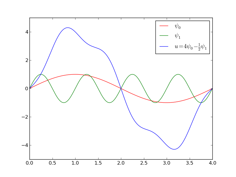
General idea of finding an approximation \( u(x) \) to some given \( f(x) \):
$$
\begin{equation}
u(x) = \sum_{i=0}^N c_i\baspsi_i(x)
\tag{1}
\end{equation}
$$
where
We shall address three approaches:
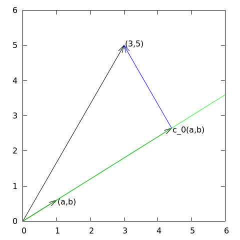
Given a vector \( \f = (3,5) \), find an approximation to \( \f \) directed along a given line.
$$
\begin{equation}
V = \mbox{span}\,\{ \psib_0\}
\end{equation}
$$
Define
$$
\begin{equation*}
\frac{\partial E}{\partial c_0} = 0
\end{equation*}
$$
$$
\begin{equation}
E(c_0) = (\e,\e) = (\f,\f) - 2c_0(\f,\psib_0) + c_0^2(\psib_0,\psib_0)
\end{equation}
$$
$$
\begin{equation}
\frac{\partial E}{\partial c_0} = -2(\f,\psib_0) + 2c_0 (\psib_0,\psib_0) = 0
\tag{2}
\end{equation}
$$
$$
\begin{equation}
c_0 = \frac{(\f,\psib_0)}{(\psib_0,\psib_0)}
\tag{3}
\end{equation}
$$
$$
\begin{equation}
c_0 = \frac{3a + 5b}{a^2 + b^2}
\end{equation}
$$
Observation for later: the vanishing derivative (2) can be alternatively written as
$$
\begin{equation}
(\e, \psib_0) = 0
\tag{4}
\end{equation}
$$
Given a vector \( \f \), find an approximation \( \u\in V \):
$$
\begin{equation*}
V = \hbox{span}\,\{\psib_0,\ldots,\psib_N\}
\end{equation*}
$$
Idea: find \( c_0,\ldots,c_N \) such that \( E= ||\e||^2 \) is minimized, \( \e=\f-\u \).
$$
\begin{align*}
E(c_0,\ldots,c_N) &= (\e,\e) = (\f -\sum_jc_j\psib_j,\f -\sum_jc_j\psib_j)
\nonumber\\
&= (\f,\f) - 2\sum_{j=0}^Nc_j(\f,\psib_j) +
\sum_{p=0}^N\sum_{q=0}^N c_pc_q(\psib_p,\psib_q)
\end{align*}
$$
$$
\begin{equation*}
\frac{\partial E}{\partial c_i} = 0,\quad i=0,\ldots,N
\end{equation*}
$$
After some work we end up with a linear system
$$
\begin{align}
\sum_{j=0}^N A_{i,j}c_j &= b_i,\quad i=0,\ldots,N\\
A_{i,j} &= (\psib_i,\psib_j)\\
b_i &= (\psib_i, \f)
\end{align}
$$
Can be shown that minimizing \( ||\e|| \) implies that \( \e \) is orthogonal to all \( \v\in V \):
$$
(\e,\v)=0,\quad \forall\v\in V
$$
which implies that \( \e \) most be orthogonal to each basis vector:
$$
\begin{equation}
(\e,\psib_i)=0,\quad i=0,\ldots,N
\tag{5}
\end{equation}
$$
This orthogonality condition is the principle of the projection (or Galerkin) method. Leads to the same linear system as in the least squares method.
Let \( V \) be a function space spanned by a set of basis functions \( \baspsi_0,\ldots,\baspsi_N \),
$$
\begin{equation*}
V = \hbox{span}\,\{\baspsi_0,\ldots,\baspsi_N\}
\end{equation*}
$$
Find \( u\in V \) as a linear combination of the basis functions:
$$
\begin{equation}
u = \sum_{j\in\If} c_j\baspsi_j,\quad\If = \{0,1,\ldots,N\}
\tag{6}
\end{equation}
$$
$$
\begin{equation}
E = (e,e) = (f-u,f-u) = (f(x)-\sum_{j\in\If} c_j\baspsi_j(x), f(x)-\sum_{j\in\If} c_j\baspsi_j(x))
\tag{7}
\end{equation}
$$
$$
\begin{equation}
E(c_0,\ldots,c_N) = (f,f) -2\sum_{j\in\If} c_j(f,\baspsi_i)
+ \sum_{p\in\If}\sum_{q\in\If} c_pc_q(\baspsi_p,\baspsi_q)
\end{equation}
$$
$$
\begin{equation*}
\frac{\partial E}{\partial c_i} = 0,\quad i=\in\If
\end{equation*}
$$
After computations identical to the vector case, we get a linear system
$$
\begin{align}
\sum_{j\in\If}^N A_{i,j}c_j &= b_i,\quad i\in\If
\tag{8}\\
A_{i,j} &= (\baspsi_i,\baspsi_j)
\tag{9}\\
b_i &= (f,\baspsi_i)
\tag{10}
\end{align}
$$
As before, minimizing \( (e,e) \) is equivalent to the projection (or Galerkin) method
$$
\begin{equation}
(e,v)=0,\quad\forall v\in V
\tag{11}
\end{equation}
$$
which means, as before,
$$
\begin{equation}
(e,\baspsi_i)=0,\quad i\in\If
\tag{12}
\end{equation}
$$
With the same algebra as in the multi-dimensional vector case, we get the same linear system as arose from the least squares method.
$$
\begin{equation*} V = \hbox{span}\,\{1, x\} \end{equation*}
$$
That is, \( \baspsi_0(x)=1 \), \( \baspsi_1(x)=x \), and \( N=1 \).
We seek
$$
\begin{equation*}
u=c_0\baspsi_0(x) + c_1\baspsi_1(x) = c_0 + c_1x
\end{equation*}
$$
$$
\begin{align}
A_{0,0} &= (\baspsi_0,\baspsi_0) = \int_1^21\cdot 1\, dx = 1\\
A_{0,1} &= (\baspsi_0,\baspsi_1) = \int_1^2 1\cdot x\, dx = 3/2\\
A_{1,0} &= A_{0,1} = 3/2\\
A_{1,1} &= (\baspsi_1,\baspsi_1) = \int_1^2 x\cdot x\,dx = 7/3
\end{align}
$$
$$
\begin{align}
b_1 &= (f,\baspsi_0) = \int_1^2 (10(x-1)^2 - 1)\cdot 1 \, dx = 7/3\\
b_2 &= (f,\baspsi_1) = \int_1^2 (10(x-1)^2 - 1)\cdot x\, dx = 13/3
\end{align}
$$
Solution of 2x2 linear system:
$$
\begin{equation}
c_0 = -38/3,\quad c_1 = 10,\quad u(x) = 10x - \frac{38}{3}
\end{equation}
$$
Consider symbolic computation of the linear system, where
sympy expression f (involving
the symbol x),psi is a list of \( \sequencei{\baspsi} \),Omega is a 2-tuple/list holding the domain \( \Omega \)Carry out the integrations, solve the linear system, and return \( u(x)=\sum_jc_j\baspsi_j(x) \)
import sympy as sp

def least_squares(f, psi, Omega):
    N = len(psi) - 1
    A = sp.zeros((N+1, N+1))
    b = sp.zeros((N+1, 1))
    x = sp.Symbol('x')
    for i in range(N+1):
        for j in range(i, N+1):
            A[i,j] = sp.integrate(psi[i]*psi[j],
                                  (x, Omega[0], Omega[1]))
            A[j,i] = A[i,j]
        b[i,0] = sp.integrate(psi[i]*f, (x, Omega[0], Omega[1]))
    c = A.LUsolve(b)
    u = 0
    for i in range(len(psi)):
        u += c[i,0]*psi[i]
    return u, c
Observe: symmetric coefficient matrix so we can halve the integrations.
f(x), psi(x,i), and a mesh x
def least_squares_numerical(f, psi, N, x,
                            integration_method='scipy',
                            orthogonal_basis=False):
    import scipy.integrate
    A = np.zeros((N+1, N+1))
    b = np.zeros(N+1)
    Omega = [x[0], x[-1]]
    dx = x[1] - x[0]

    for i in range(N+1):
        j_limit = i+1 if orthogonal_basis else N+1
        for j in range(i, j_limit):
            print '(%d,%d)' % (i, j)
            if integration_method == 'scipy':
                A_ij = scipy.integrate.quad(
                    lambda x: psi(x,i)*psi(x,j),
                    Omega[0], Omega[1], epsabs=1E-9, epsrel=1E-9)[0]
            elif ...
            A[i,j] = A[j,i] = A_ij

        if integration_method == 'scipy':
            b_i = scipy.integrate.quad(
                lambda x: f(x)*psi(x,i), Omega[0], Omega[1],
                epsabs=1E-9, epsrel=1E-9)[0]
        elif ...
        b[i] = b_i

    c = b/np.diag(A) if orthogonal_basis else np.linalg.solve(A, b)
    u = sum(c[i]*psi(x, i) for i in range(N+1))
    return u, c
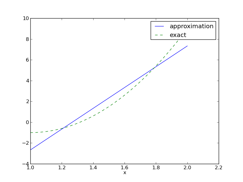
Compare \( f \) and \( u \) visually:
def comparison_plot(f, u, Omega, filename='tmp.pdf'):
    x = sp.Symbol('x')
    # Turn f and u to ordinary Python functions
    f = sp.lambdify([x], f, modules="numpy")
    u = sp.lambdify([x], u, modules="numpy")
    resolution = 401  # no of points in plot
    xcoor  = linspace(Omega[0], Omega[1], resolution)
    exact  = f(xcoor)
    approx = u(xcoor)
    plot(xcoor, approx)
    hold('on')
    plot(xcoor, exact)
    legend(['approximation', 'exact'])
    savefig(filename)
All code in module approx1D.py
>>> from approx1D import *
>>> x = sp.Symbol('x')
>>> f = 10*(x-1)**2-1
>>> u, c = least_squares(f=f, psi=[1, x], Omega=[1, 2])
>>> comparison_plot(f, u, Omega=[1, 2])
>>> from approx1D import *
>>> x = sp.Symbol('x')
>>> f = 10*(x-1)**2-1
>>> u, c = least_squares(f=f, psi=[1, x, x**2], Omega=[1, 2])
>>> print u
10*x**2 - 20*x + 9
>>> print sp.expand(f)
10*x**2 - 20*x + 9
least_squares is \( c_i=0 \) for \( i>2 \)
If \( f\in V \), \( f=\sum_{j\in\If}d_j\baspsi_j \), for some \( \sequencei{d} \). Then
$$
\begin{equation*}
b_i = (f,\baspsi_i) = \sum_{j\in\If}d_j(\baspsi_j, \baspsi_i)
= \sum_{j\in\If} d_jA_{i,j}
\end{equation*}
$$
The linear system \( \sum_j A_{i,j}c_j = b_i \), \( i\in\If \), is then
$$
\begin{equation*}
\sum_{j\in\If}c_jA_{i,j} = \sum_{j\in\If}d_jA_{i,j},\quad i\in\If
\end{equation*}
$$
which implies that \( c_i=d_i \) for \( i\in\If \) and \( u \) is identical to \( f \).
The previous computations were symbolic. What if we solve the linear system numerically with standard arrays?
| exact | sympy | numpy32 | numpy64 |
| 9 | 9.62 | 5.57 | 8.98 |
| -20 | -23.39 | -7.65 | -19.93 |
| 10 | 17.74 | -4.50 | 9.96 |
| 0 | -9.19 | 4.13 | -0.26 |
| 0 | 5.25 | 2.99 | 0.72 |
| 0 | 0.18 | -1.21 | -0.93 |
| 0 | -2.48 | -0.41 | 0.73 |
| 0 | 1.81 | -0.013 | -0.36 |
| 0 | -0.66 | 0.08 | 0.11 |
| 0 | 0.12 | 0.04 | -0.02 |
| 0 | -0.001 | -0.02 | 0.002 |
sympy.mpmath.fp.matrix and sympy.mpmath.fp.lu_solvenumpy arrays with numpy.float32 entriesnumpy arrays with numpy.float64 entries
Observations:
Problem: The basis functions \( x^i \) become almost linearly dependent for large \( N \).
Consider
$$
\begin{equation*}
V = \hbox{span}\,\{ \sin \pi x, \sin 2\pi x,\ldots,\sin (N+1)\pi x\}
\end{equation*}
$$
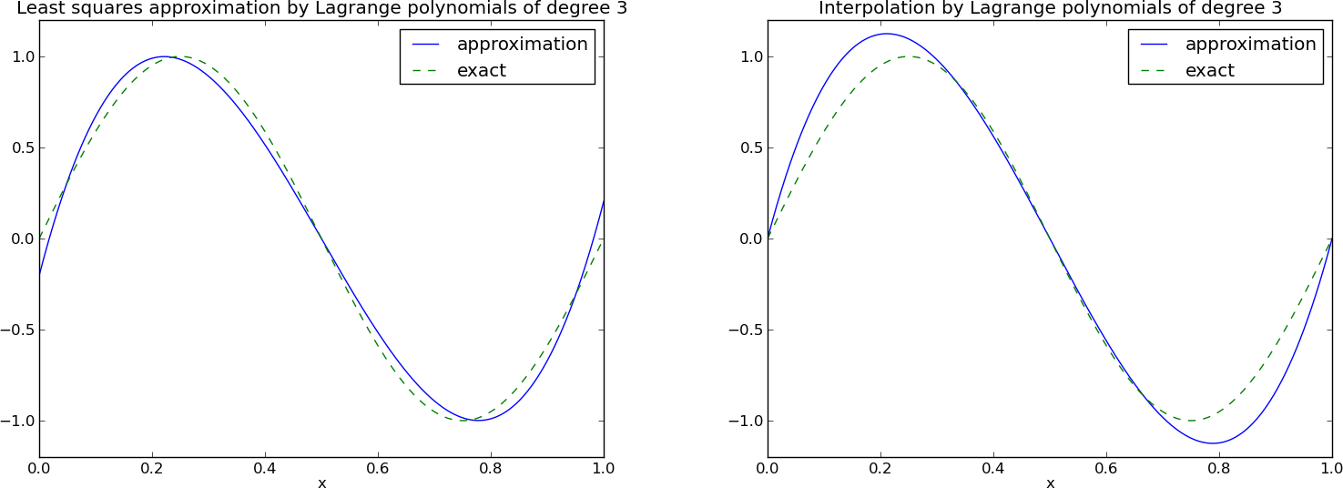
N = 3
from sympy import sin, pi
psi = [sin(pi*(i+1)*x) for i in range(N+1)]
f = 10*(x-1)**2 - 1
Omega = [0, 1]
u, c = least_squares(f, psi, Omega)
comparison_plot(f, u, Omega)
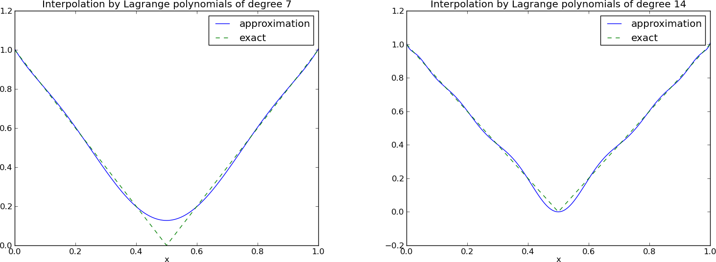
\( N=3 \) vs \( N=11 \):

$$
\begin{equation}
u(x) = f(0)(1-x) + xf(1) + \sum_{j\in\If} c_j\baspsi_j(x)
\end{equation}
$$
The extra term ensures \( u(0)=f(0) \) and \( u(1)=f(1) \) and
is a strikingly good help to get a good
approximation!
\( N=3 \) vs \( N=11 \):

This choice of sine functions as basis functions is popular because
In general for an orthogonal basis, \( A_{i,j} \) is diagonal and we can easily solve for \( c_i \):
$$
c_i = \frac{b_i}{A_{i,i}} = \frac{(f,\baspsi_i)}{(\baspsi_i,\baspsi_i)}
$$
Here is another idea for approximating \( f(x) \) by \( u(x)=\sum_jc_j\baspsi_j \):
$$
\begin{equation}
u(\xno{i}) = \sum_{j\in\If} c_j \baspsi_j(\xno{i}) = f(\xno{i})
\quad i\in\If,N
\end{equation}
$$
This is a linear system with no need for integration:
$$
\begin{align}
\sum_{j\in\If} A_{i,j}c_j &= b_i,\quad i\in\If\\
A_{i,j} &= \baspsi_j(\xno{i})\\
b_i &= f(\xno{i})
\end{align}
$$
No symmetric matrix: \( \baspsi_j(\xno{i})\neq \baspsi_i(\xno{j}) \) in general
points holds the interpolation/collocation points
def interpolation(f, psi, points):
    N = len(psi) - 1
    A = sp.zeros((N+1, N+1))
    b = sp.zeros((N+1, 1))
    x = sp.Symbol('x')
    # Turn psi and f into Python functions
    psi = [sp.lambdify([x], psi[i]) for i in range(N+1)]
    f = sp.lambdify([x], f)
    for i in range(N+1):
        for j in range(N+1):
            A[i,j] = psi[j](points[i])
        b[i,0] = f(points[i])
    c = A.LUsolve(b)
    u = 0
    for i in range(len(psi)):
        u += c[i,0]*psi[i](x)
    return u
\( (4/3,5/3) \) vs \( (1,2) \):

Motivation:
The Lagrange interpolating polynomials \( \baspsi_j \) have the property that
$$ \baspsi_i(\xno{j}) =\delta_{ij},\quad \delta_{ij} =
\left\lbrace\begin{array}{ll}
1, & i=j\\
0, & i\neq j
\end{array}\right.
$$
Hence, \( c_i = f(x_i) \) and
$$
\begin{equation}
u(x) = \sum_{j\in\If} f(\xno{i})\baspsi_i(x)
\end{equation}
$$
$$
\begin{equation}
\baspsi_i(x) =
\prod_{j=0,j\neq i}^N
\frac{x-\xno{j}}{\xno{i}-\xno{j}}
= \frac{x-x_0}{\xno{i}-x_0}\cdots\frac{x-\xno{i-1}}{\xno{i}-\xno{i-1}}\frac{x-\xno{i+1}}{\xno{i}-\xno{i+1}}
\cdots\frac{x-x_N}{\xno{i}-x_N}
\tag{13}
\end{equation}
$$
def Lagrange_polynomial(x, i, points):
    p = 1
    for k in range(len(points)):
        if k != i:
            p *= (x - points[k])/(points[i] - points[k])
    return p

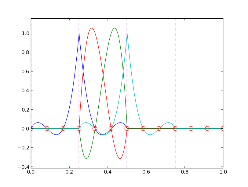
12 points, degree 11, plot of two of the Lagrange polynomials - note that they are zero at all points except one.

Problem: strong oscillations near the boundaries for larger \( N \) values.
The oscillations can be reduced by a more clever choice of interpolation points, called the Chebyshev nodes:
$$
\begin{equation}
\xno{i} = \half (a+b) + \half(b-a)\cos\left( \frac{2i+1}{2(N+1)}pi\right),\quad i=0\ldots,N
\end{equation}
$$
on an interval \( [a,b] \).
12 points, degree 11, plot of two of the Lagrange polynomials - note that they are zero at all points except one.


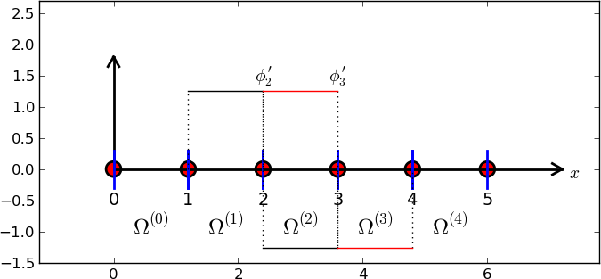
Split \( \Omega \) into non-overlapping subdomains called elements:
$$
\begin{equation}
\Omega = \Omega^{(0)}\cup \cdots \cup \Omega^{(N_e)}
\end{equation}
$$
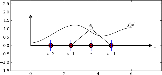
On each element, introduce points called nodes: \( \xno{0},\ldots,\xno{N_n} \)
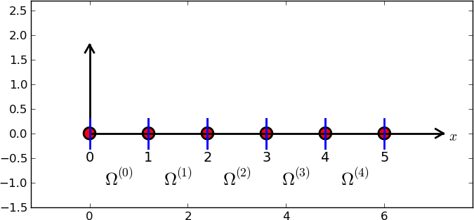
Data structure: nodes holds coordinates or nodes, elements holds the
node numbers in each element
nodes = [0, 1.2, 2.4, 3.6, 4.8, 5]
elements = [[0, 1], [1, 2], [2, 3], [3, 4], [4, 5]]
nodes = [0, 0.125, 0.25, 0.375, 0.5, 0.625, 0.75, 0.875, 1.0]
elements = [[0, 1, 2], [2, 3, 4], [4, 5, 6], [6, 7, 8]]


d = 3  # d+1 nodes per element
num_elements = 4
num_nodes = num_elements*d + 1
nodes = [i*0.5 for i in range(num_nodes)]
elements = [[i*d+j for j in range(d+1)] for i in range(num_elements)]
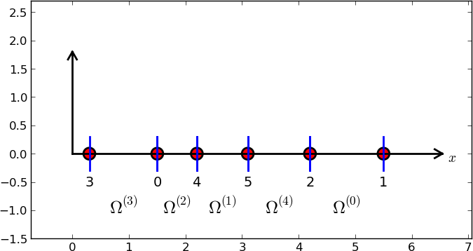
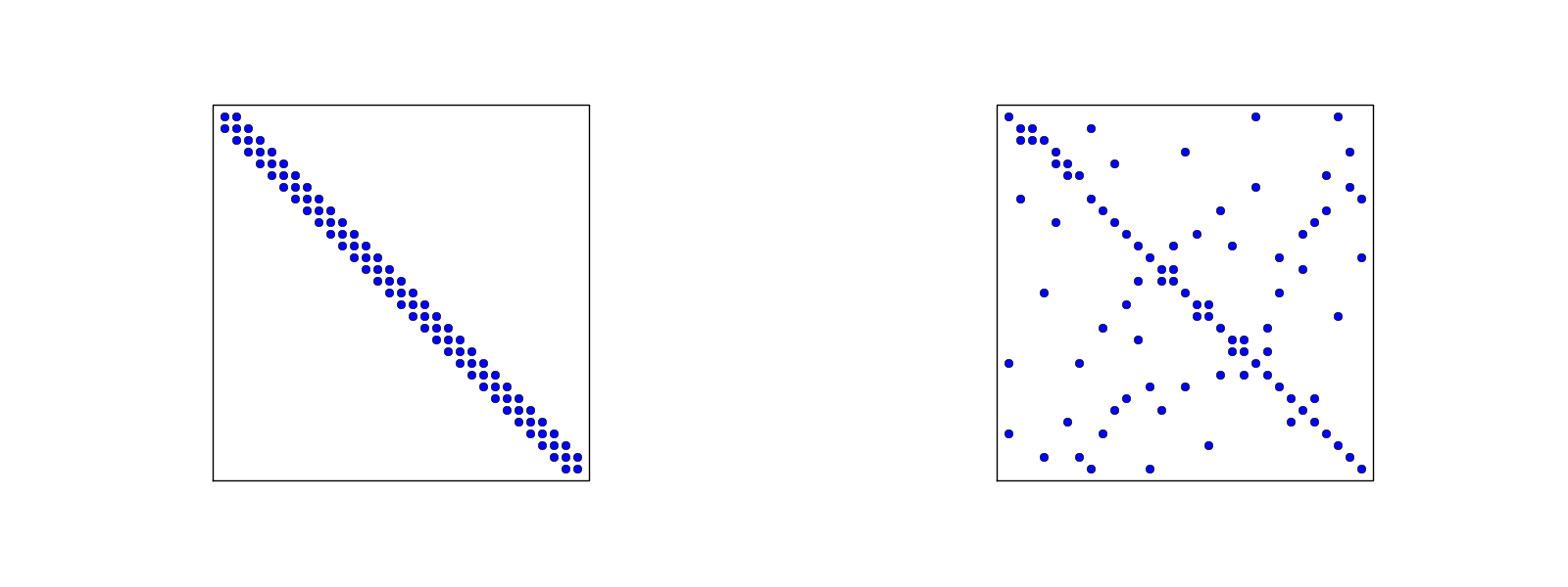
nodes = [1.5, 5.5, 4.2, 0.3, 2.2, 3.1]
elements = [[2, 1], [4, 5], [0, 4], [3, 0], [5, 2]]
Important property: \( c_i \) is the value of \( u \) at node \( i \), \( \xno{i} \):
$$
\begin{equation}
u(\xno{i}) = \sum_{j\in\If} c_j\basphi_j(\xno{i}) =
c_i\basphi_i(\xno{i}) = c_i
\tag{14}
\end{equation}
$$
because \( \basphi_j(\xno{i}) =0 \) if \( i\neq j \)
Since \( A_{i,j}=\int\basphi_i\basphi_j\dx \), most of the elements in the coefficient matrix will be zero
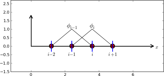
$$
\begin{equation}
\basphi_i(x) = \left\lbrace\begin{array}{ll}
0, & x < \xno{i-1}\\
(x - \xno{i-1})/h
& \xno{i-1} \leq x < \xno{i}\\
1 -
(x - x_{i})/h,
& \xno{i} \leq x < \xno{i+1}\\
0, & x\geq \xno{i+1}
\end{array}
\right.
\tag{15}
\end{equation}
$$
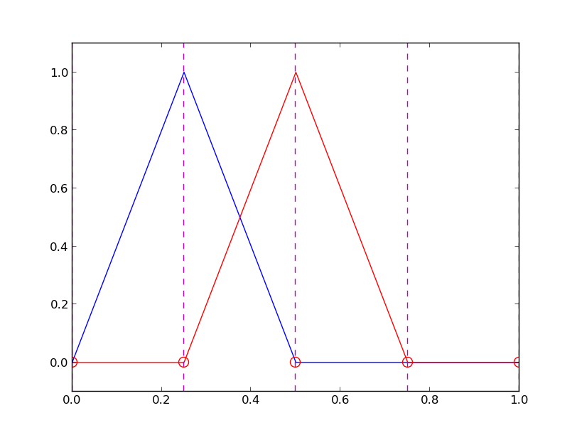
\( A_{2,3}=\int_\Omega\basphi_2\basphi_3 dx \): \( \basphi_2\basphi_3\neq 0 \) only over element 2. There,
$$ \basphi_3(x) = (x-x_2)/h,\quad \basphi_2(x) = 1- (x-x_2)/h$$
$$
A_{2,3} = \int_\Omega \basphi_2\basphi_{3}\dx =
\int_{\xno{2}}^{\xno{3}}
\left(1 - \frac{x - \xno{2}}{h}\right) \frac{x - x_{2}}{h}
\dx = \frac{h}{6}
$$
$$ A_{2,2} =
\int_{\xno{1}}^{\xno{2}}
\left(\frac{x - \xno{1}}{h}\right)^2\dx +
\int_{\xno{2}}^{\xno{3}}
\left(1 - \frac{x - \xno{2}}{h}\right)^2\dx
= \frac{h}{3}
$$
$$ A_{i,i-1} = \int_\Omega \basphi_i\basphi_{i-1}\dx = \hbox{?}$$
$$
\begin{align*}
A_{i,i-1} &= \int_\Omega \basphi_i\basphi_{i-1}\dx\\
&=
\underbrace{\int_{\xno{i-2}}^{\xno{i-1}} \basphi_i\basphi_{i-1}\dx}_{\basphi_i=0} +
\int_{\xno{i-1}}^{\xno{i}} \basphi_i\basphi_{i-1}\dx +
\underbrace{\int_{\xno{i}}^{\xno{i+1}} \basphi_i\basphi_{i-1}\dx}_{\basphi_{i-1}=0}\\
&= \int_{\xno{i-1}}^{\xno{i}}
\underbrace{\left(\frac{x - x_{i}}{h}\right)}_{\basphi_i(x)}
\underbrace{\left(1 - \frac{x - \xno{i-1}}{h}\right)}_{\basphi_{i-1}(x)} \dx =
\frac{h}{6}
\end{align*}
$$
$$
\begin{equation}
b_i = \int_\Omega\basphi_i(x)f(x)\dx
= \int_{\xno{i-1}}^{\xno{i}} \frac{x - \xno{i-1}}{h} f(x)\dx
+ \int_{x_{i}}^{\xno{i+1}} \left(1 - \frac{x - x_{i}}{h}\right) f(x)
\dx
\tag{16}
\end{equation}
$$
Need a specific \( f(x) \) to do more...
$$
\begin{equation*}
A = \frac{h}{6}\left(\begin{array}{ccc}
2 & 1 & 0\\
1 & 4 & 1\\
0 & 1 & 2
\end{array}\right),\quad
b = \frac{h^2}{12}\left(\begin{array}{c}
2 - 3h\\
12 - 14h\\
10 -17h
\end{array}\right)
\end{equation*}
$$
$$
\begin{equation*} c_0 = \frac{h^2}{6},\quad c_1 = h - \frac{5}{6}h^2,\quad
c_2 = 2h - \frac{23}{6}h^2
\end{equation*}
$$
$$
\begin{equation*} u(x)=c_0\basphi_0(x) + c_1\basphi_1(x) + c_2\basphi_2(x)\end{equation*}
$$


$$
\begin{equation}
A_{i,j} = \int_\Omega\basphi_i\basphi_jdx =
\sum_{e} \int_{\Omega^{(e)}} \basphi_i\basphi_jdx,\quad
A^{(e)}_{i,j}=\int_{\Omega^{(e)}} \basphi_i\basphi_jdx
\tag{17}
\end{equation}
$$
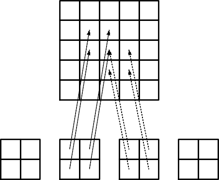
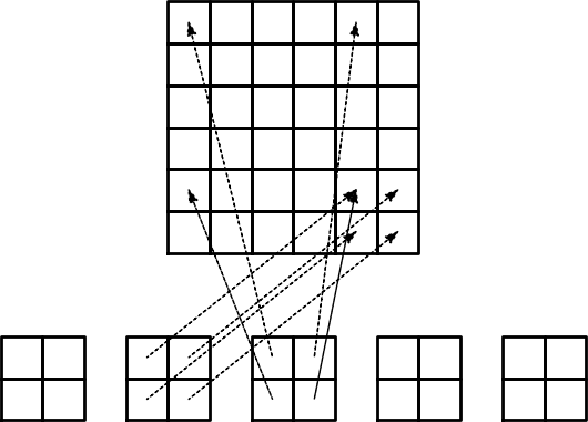
Important:
$$
\tilde A^{(e)} = \{ \tilde A^{(e)}_{r,s}\},\quad
\tilde A^{(e)}_{r,s} =
\int_{\Omega^{(e)}}\basphi_{q(e,r)}\basphi_{q(e,s)}dx,
\quad r,s\in\Ifd=\{0,\ldots,d\}
$$
i=elements[e][r])
$$
\begin{equation}
A_{q(e,r),q(e,s)} := A_{q(e,r),q(e,s)} + \tilde A^{(e)}_{r,s},\quad
r,s\in\Ifd
\end{equation}
$$

$$
\begin{equation}
b_i = \int_\Omega f(x)\basphi_i(x)dx =
\sum_{e} \int_{\Omega^{(e)}} f(x)\basphi_i(x)dx,\quad
b^{(e)}_{i}=\int_{\Omega^{(e)}} f(x)\basphi_i(x)dx
\end{equation}
$$
Important:
Assembly:
$$
\begin{equation}
b_{q(e,r)} := b_{q(e,r)} + \tilde b^{(e)}_{r},\quad
r,s\in\Ifd
\end{equation}
$$
Instead of computing
$$
\begin{equation*} \tilde A^{(e)}_{r,s} = \int_{\Omega^{(e)}}\basphi_{q(e,r)}(x)\basphi_{q(e,s)}(x)dx
= \int_{x_L}^{x_R}\basphi_{q(e,r)}(x)\basphi_{q(e,s)}(x)dx
\end{equation*}
$$
we now map \( [x_L, x_R] \) to
a standardized reference element domain \( [-1,1] \) with local coordinate \( X \)
$$
\begin{equation}
x = \half (x_L + x_R) + \half (x_R - x_L)X
\tag{18}
\end{equation}
$$
or rewritten as
$$
\begin{equation}
x = x_m + {\half}hX, \qquad x_m=(x_L+x_R)/2
\tag{19}
\end{equation}
$$
Reference element integration: just change integration variable from \( x \) to \( X \). Introduce local basis function
$$
\begin{equation}
\refphi_r(X) = \basphi_{q(e,r)}(x(X))
\end{equation}
$$
$$
\begin{equation}
\tilde A^{(e)}_{r,s} = \int_{\Omega^{(e)}}\basphi_{q(e,r)}(x)\basphi_{q(e,s)}(x)dx
= \int\limits_{-1}^1 \refphi_r(X)\refphi_s(X)\underbrace{\frac{dx}{dX}}_{\det J = h/2}dX
= \int\limits_{-1}^1 \refphi_r(X)\refphi_s(X)\det J\,dX
\end{equation}
$$
$$
\begin{equation}
\tilde b^{(e)}_{r} = \int_{\Omega^{(e)}}f(x)\basphi_{q(e,r)}(x)dx
= \int\limits_{-1}^1 f(x(X))\refphi_r(X)\det J\,dX
\tag{20}
\end{equation}
$$
$$
\begin{align}
\refphi_0(X) &= \half (1 - X)
\tag{21}\\
\refphi_1(X) &= \half (1 + X)
\tag{22}
\end{align}
$$
P2 elements:
$$
\begin{align}
\refphi_0(X) &= \half (X-1)X\\
\refphi_1(X) &= 1 - X^2\\
\refphi_2(X) &= \half (X+1)X
\end{align}
$$
Easy to generalize to arbitrary order!
P1 elements and \( f(x)=x(1-x) \).
$$
\begin{align}
\tilde A^{(e)}_{0,0}
&= \int_{-1}^1 \refphi_0(X)\refphi_0(X)\frac{h}{2} dX\nonumber\\
&=\int_{-1}^1 \half(1-X)\half(1-X) \frac{h}{2} dX =
\frac{h}{8}\int_{-1}^1 (1-X)^2 dX = \frac{h}{3}
\tag{23}\\
\tilde A^{(e)}_{1,0}
&= \int_{-1}^1 \refphi_1(X)\refphi_0(X)\frac{h}{2} dX\nonumber\\
&=\int_{-1}^1 \half(1+X)\half(1-X) \frac{h}{2} dX =
\frac{h}{8}\int_{-1}^1 (1-X^2) dX = \frac{h}{6}\\
\tilde A^{(e)}_{0,1} &= \tilde A^{(e)}_{1,0}
\tag{24}\\
\tilde A^{(e)}_{1,1}
&= \int_{-1}^1 \refphi_1(X)\refphi_1(X)\frac{h}{2} dX\nonumber\\
&=\int_{-1}^1 \half(1+X)\half(1+X) \frac{h}{2} dX =
\frac{h}{8}\int_{-1}^1 (1+X)^2 dX = \frac{h}{3}
\tag{25}
\end{align}
$$
$$
\begin{align}
\tilde b^{(e)}_{0}
&= \int_{-1}^1 f(x(X))\refphi_0(X)\frac{h}{2} dX\nonumber\\
&= \int_{-1}^1 (x_m + \half hX)(1-(x_m + \half hX))
\half(1-X)\frac{h}{2} dX \nonumber\\
&= - \frac{1}{24} h^{3} + \frac{1}{6} h^{2} x_{m} - \frac{1}{12} h^{2} - \half h x_{m}^{2} + \half h x_{m}
\tag{26}\\
\tilde b^{(e)}_{1}
&= \int_{-1}^1 f(x(X))\refphi_1(X)\frac{h}{2} dX\nonumber\\
&= \int_{-1}^1 (x_m + \half hX)(1-(x_m + \half hX))
\half(1+X)\frac{h}{2} dX \nonumber\\
&= - \frac{1}{24} h^{3} - \frac{1}{6} h^{2} x_{m} + \frac{1}{12} h^{2} -
\half h x_{m}^{2} + \half h x_{m}
\end{align}
$$
\( x_m \): element midpoint.
>>> import sympy as sp
>>> x, x_m, h, X = sp.symbols('x x_m h X')
>>> sp.integrate(h/8*(1-X)**2, (X, -1, 1))
h/3
>>> sp.integrate(h/8*(1+X)*(1-X), (X, -1, 1))
h/6
>>> x = x_m + h/2*X
>>> b_0 = sp.integrate(h/4*x*(1-x)*(1-X), (X, -1, 1))
>>> print b_0
-h**3/24 + h**2*x_m/6 - h**2/12 - h*x_m**2/2 + h*x_m/2
Can printe out in LaTeX too (convenient for copying into reports):
>>> print sp.latex(b_0, mode='plain')
- \frac{1}{24} h^{3} + \frac{1}{6} h^{2} x_{m}
- \frac{1}{12} h^{2} - \half h x_{m}^{2}
+ \half h x_{m}
Let \( \refphi_r(X) \) be a Lagrange polynomial of degree d:
import sympy as sp
import numpy as np

def phi_r(r, X, d):
    if isinstance(X, sp.Symbol):
        h = sp.Rational(1, d)  # node spacing
        nodes = [2*i*h - 1 for i in range(d+1)]
    else:
        # assume X is numeric: use floats for nodes
        nodes = np.linspace(-1, 1, d+1)
    return Lagrange_polynomial(X, r, nodes)

def Lagrange_polynomial(x, i, points):
    p = 1
    for k in range(len(points)):
        if k != i:
            p *= (x - points[k])/(points[i] - points[k])
    return p

def basis(d=1):
    """Return the complete basis."""
    X = sp.Symbol('X')
    phi = [phi_r(r, X, d) for r in range(d+1)]
    return phi
def element_matrix(phi, Omega_e, symbolic=True):
    n = len(phi)
    A_e = sp.zeros((n, n))
    X = sp.Symbol('X')
    if symbolic:
        h = sp.Symbol('h')
    else:
        h = Omega_e[1] - Omega_e[0]
    detJ = h/2  # dx/dX
    for r in range(n):
        for s in range(r, n):
            A_e[r,s] = sp.integrate(phi[r]*phi[s]*detJ, (X, -1, 1))
            A_e[s,r] = A_e[r,s]
    return A_e
>>> from fe_approx1D import *
>>> phi = basis(d=1)
>>> phi
[1/2 - X/2, 1/2 + X/2]
>>> element_matrix(phi, Omega_e=[0.1, 0.2], symbolic=True)
[h/3, h/6]
[h/6, h/3]
>>> element_matrix(phi, Omega_e=[0.1, 0.2], symbolic=False)
[0.0333333333333333, 0.0166666666666667]
[0.0166666666666667, 0.0333333333333333]
def element_vector(f, phi, Omega_e, symbolic=True):
    n = len(phi)
    b_e = sp.zeros((n, 1))
    # Make f a function of X
    X = sp.Symbol('X')
    if symbolic:
        h = sp.Symbol('h')
    else:
        h = Omega_e[1] - Omega_e[0]
    x = (Omega_e[0] + Omega_e[1])/2 + h/2*X  # mapping
    f = f.subs('x', x)  # substitute mapping formula for x
    detJ = h/2  # dx/dX
    for r in range(n):
        b_e[r] = sp.integrate(f*phi[r]*detJ, (X, -1, 1))
    return b_e
Note f.subs('x', x): replace x by \( x(X) \) such that f contains X
sympy always succeedssympy then returns an Integral object instead of a number)
def element_vector(f, phi, Omega_e, symbolic=True):
        ...
        I = sp.integrate(f*phi[r]*detJ, (X, -1, 1))  # try...
        if isinstance(I, sp.Integral):
            h = Omega_e[1] - Omega_e[0]  # Ensure h is numerical
            detJ = h/2
            integrand = sp.lambdify([X], f*phi[r]*detJ)
            I = sp.mpmath.quad(integrand, [-1, 1])
        b_e[r] = I
        ...
def assemble(nodes, elements, phi, f, symbolic=True):
    N_n, N_e = len(nodes), len(elements)
    zeros = sp.zeros if symbolic else np.zeros
    A = zeros((N_n, N_n))
    b = zeros((N_n, 1))
    for e in range(N_e):
        Omega_e = [nodes[elements[e][0]], nodes[elements[e][-1]]]

        A_e = element_matrix(phi, Omega_e, symbolic)
        b_e = element_vector(f, phi, Omega_e, symbolic)

        for r in range(len(elements[e])):
            for s in range(len(elements[e])):
                A[elements[e][r],elements[e][s]] += A_e[r,s]
            b[elements[e][r]] += b_e[r]
    return A, b
if symbolic:
    c = A.LUsolve(b)           # sympy arrays, symbolic Gaussian elim.
else:
    c = np.linalg.solve(A, b)  # numpy arrays, numerical solve
Note: the symbolic computation of A and b and the symbolic
solution can be very tedious.
>>> h, x = sp.symbols('h x')
>>> nodes = [0, h, 2*h]
>>> elements = [[0, 1], [1, 2]]
>>> phi = basis(d=1)
>>> f = x*(1-x)
>>> A, b = assemble(nodes, elements, phi, f, symbolic=True)
>>> A
[h/3,   h/6,   0]
[h/6, 2*h/3, h/6]
[  0,   h/6, h/3]
>>> b
[     h**2/6 - h**3/12]
[      h**2 - 7*h**3/6]
[5*h**2/6 - 17*h**3/12]
>>> c = A.LUsolve(b)
>>> c
[                           h**2/6]
[12*(7*h**2/12 - 35*h**3/72)/(7*h)]
[  7*(4*h**2/7 - 23*h**3/21)/(2*h)]
>>> nodes = [0, 0.5, 1]
>>> elements = [[0, 1], [1, 2]]
>>> phi = basis(d=1)
>>> x = sp.Symbol('x')
>>> f = x*(1-x)
>>> A, b = assemble(nodes, elements, phi, f, symbolic=False)
>>> A
[ 0.166666666666667, 0.0833333333333333,                  0]
[0.0833333333333333,  0.333333333333333, 0.0833333333333333]
[                 0, 0.0833333333333333,  0.166666666666667]
>>> b
[          0.03125]
[0.104166666666667]
[          0.03125]
>>> c = A.LUsolve(b)
>>> c
[0.0416666666666666]
[ 0.291666666666667]
[0.0416666666666666]
>>> d=1; N_e=8; Omega=[0,1]  # 8 linear elements on [0,1]
>>> phi = basis(d)
>>> f = x*(1-x)
>>> nodes, elements = mesh_symbolic(N_e, d, Omega)
>>> A, b = assemble(nodes, elements, phi, f, symbolic=True)
>>> A
[h/3,   h/6,     0,     0,     0,     0,     0,     0,   0]
[h/6, 2*h/3,   h/6,     0,     0,     0,     0,     0,   0]
[  0,   h/6, 2*h/3,   h/6,     0,     0,     0,     0,   0]
[  0,     0,   h/6, 2*h/3,   h/6,     0,     0,     0,   0]
[  0,     0,     0,   h/6, 2*h/3,   h/6,     0,     0,   0]
[  0,     0,     0,     0,   h/6, 2*h/3,   h/6,     0,   0]
[  0,     0,     0,     0,     0,   h/6, 2*h/3,   h/6,   0]
[  0,     0,     0,     0,     0,     0,   h/6, 2*h/3, h/6]
[  0,     0,     0,     0,     0,     0,     0,   h/6, h/3]
Note: do this by hand to understand what is going on!
$$
\begin{equation}
A = \frac{h}{6}
\left(
\begin{array}{cccccccccc}
2 & 1 & 0
&\cdots & \cdots & \cdots & \cdots & \cdots & 0 \\
1 & 4 & 1 & \ddots & & & & & \vdots \\
0 & 1 & 4 & 1 &
\ddots & & & & \vdots \\
\vdots & \ddots & & \ddots & \ddots & 0 & & & \vdots \\
\vdots & & \ddots & \ddots & \ddots & \ddots & \ddots & & \vdots \\
\vdots & & & 0 & 1 & 4 & 1 & \ddots & \vdots \\
\vdots & & & & \ddots & \ddots & \ddots &\ddots & 0 \\
\vdots & & & & &\ddots & 1 & 4 & 1 \\
0 &\cdots & \cdots &\cdots & \cdots & \cdots & 0 & 1 & 2
\end{array}
\right)
\end{equation}
$$
$$
\begin{equation}
A = \frac{h}{30}
\left(
\begin{array}{ccccccccc}
4 & 2 & - 1 & 0
& 0 & 0 & 0 & 0 & 0\\
2 & 16 & 2
& 0 & 0 & 0 & 0 & 0 & 0\\- 1 & 2 &
8 & 2 & - 1 & 0 & 0 & 0 & 0\\
0 & 0 & 2 & 16 & 2 & 0 & 0 & 0 & 0\\
0 & 0 & - 1 & 2 & 8 & 2 & - 1 & 0 & 0\\
0 & 0 & 0 & 0 & 2 & 16 & 2 & 0 & 0\\
0 & 0 & 0 & 0 & - 1 & 2 & 8 & 2 & - 1
\\0 & 0 & 0 & 0 & 0 & 0 &
2 & 16 & 2\\0 & 0 & 0 & 0 & 0
& 0 & - 1 & 2 & 4
\end{array}
\right)
\end{equation}
$$
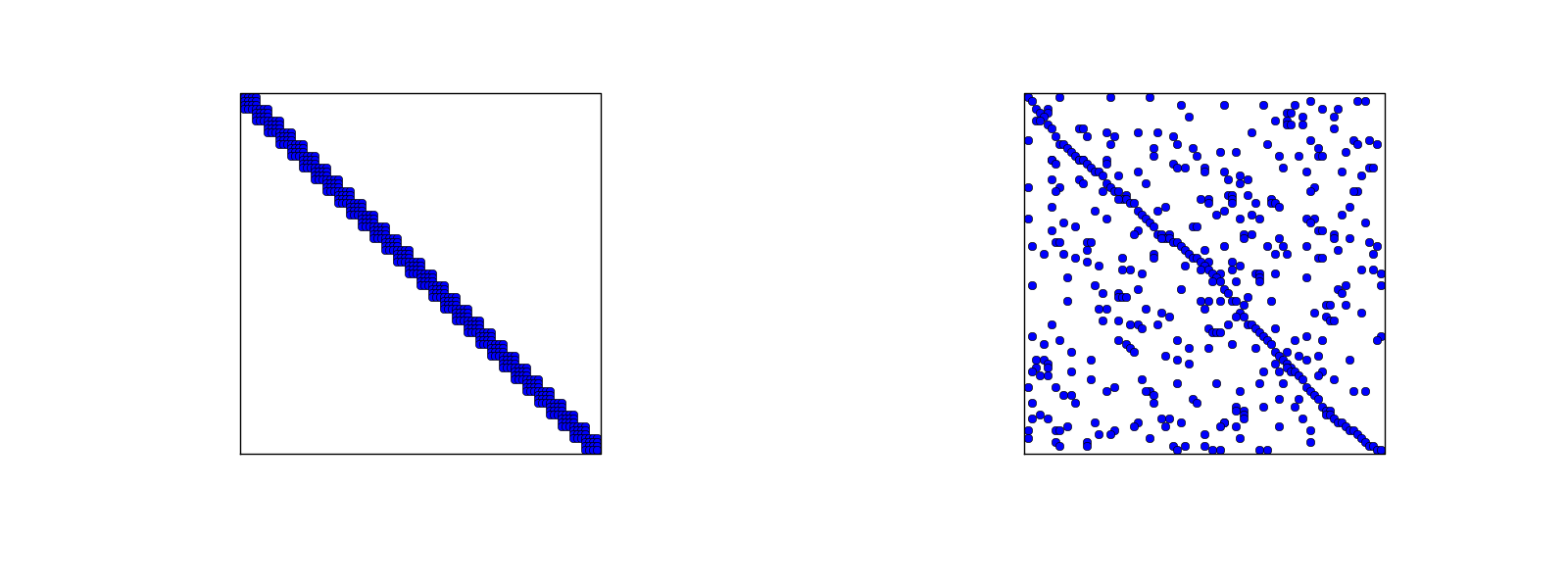
The minimum storage requirements for the coefficient matrix \( A_{i,j} \):
scipy.sparse package
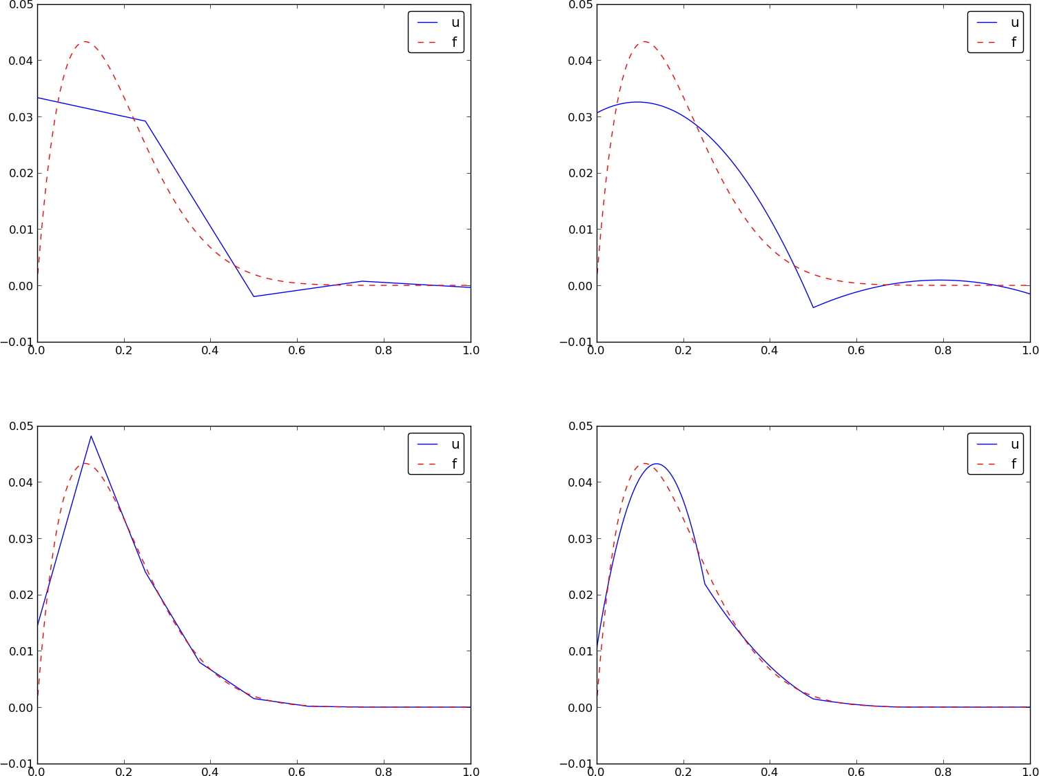
Compute a mesh with \( N_e \) elements, basis functions of degree \( d \), and approximate a given symbolic expression \( f(x) \) by a finite element expansion \( u(x) = \sum_jc_j\basphi_j(x) \):
import sympy as sp
from fe_approx1D import approximate
x = sp.Symbol('x')
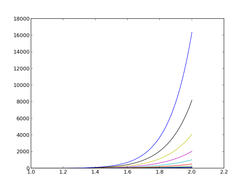
approximate(f=x*(1-x)**8, symbolic=False, d=1, N_e=4)
approximate(f=x*(1-x)**8, symbolic=False, d=2, N_e=2)
approximate(f=x*(1-x)**8, symbolic=False, d=1, N_e=8)
approximate(f=x*(1-x)**8, symbolic=False, d=2, N_e=4)
Let \( \{\xno{i}\}_{i\in\If} \) be the nodes in the mesh. Collocation means
$$
\begin{equation}
u(\xno{i})=f(\xno{i}),\quad i\in\If,
\end{equation}
$$
which translates to
$$ \sum_{j\in\If} c_j \basphi_j(\xno{i}) = f(\xno{i}),$$
but \( \basphi_j(\xno{i})=0 \) if \( i\neq j \) so the sum collapses to one
term \( c_i\basphi_i(\xno{i}) = c_i \), and we have the result
$$
\begin{equation}
c_i = f(\xno{i})
\end{equation}
$$
Same result as the standard finite difference approach, but finite elements define \( u \) also between the \( \xno{i} \) points
The P1 finite element machinery results in a linear system where equation no \( i \) is
$$
\begin{equation}
\frac{h}{6}(u_{i-1} + 4u_i + u_{i+1}) = (f,\basphi_i)
\tag{27}
\end{equation}
$$
Note:
Rewrite the left-hand side of finite element equation no \( i \):
$$
\begin{equation}
h(u_i + \frac{1}{6}(u_{i-1} - 2u_i + u_{i+1})) = [h(u + \frac{h^2}{6}D_x D_x u)]_i
\end{equation}
$$
This is the standard finite difference approximation of
$$ h(u + \frac{h^2}{6}u'')$$
$$ (f,\basphi_i) = \int_{\xno{i-1}}^{\xno{i}} f(x)\frac{1}{h} (x - \xno{i-1}) dx
+ \int_{\xno{i}}^{\xno{i+1}} f(x)\frac{1}{h}(1 - (x - x_{i})) dx
$$
Cannot do much unless we specialize \( f \) or use numerical integration.
Trapezoidal rule using the nodes:
$$ (f,\basphi_i) = \int_\Omega f\basphi_i dx\approx h\half(
f(\xno{0})\basphi_i(\xno{0}) + f(\xno{N})\basphi_i(\xno{N}))
+ h\sum_{j=1}^{N-1} f(\xno{j})\basphi_i(\xno{j})
$$
\( \basphi_i(\xno{j})=\delta_{ij} \), so this formula collapses to one term:
$$
\begin{equation}
(f,\basphi_i) \approx hf(\xno{i}),\quad i=1,\ldots,N-1\thinspace.
\end{equation}
$$
Same result as in collocation (interpolation) and the finite difference method!
$$ \int_\Omega g(x)dx \approx \frac{h}{6}\left( g(\xno{0}) +
2\sum_{j=1}^{N-1} g(\xno{j})
+ 4\sum_{j=0}^{N-1} g(\xno{j+\half}) + f(\xno{2N})\right),
$$
Our case: \( g=f\basphi_i \). The sums collapse because \( \basphi_i=0 \) at most of
the points.
$$
\begin{equation}
(f,\basphi_i) \approx \frac{h}{3}(f_{i-\half} + f_i + f_{i+\half})
\end{equation}
$$
Conclusions:
With Trapezoidal integration of \( (f,\basphi_i) \), the finite element metod essentially solve
$$
\begin{equation}
u + \frac{h^2}{6} u'' = f,\quad u'(0)=u'(L)=0,
\end{equation}
$$
by the finite difference method
$$
\begin{equation}
[u + \frac{h^2}{6} D_x D_x u = f]_i
\end{equation}
$$
With Simpson integration of \( (f,\basphi_i) \) we essentially solve
$$
\begin{equation}
[u + \frac{h^2}{6} D_x D_x u = \bar f]_i,
\end{equation}
$$
where
$$ \bar f_i = \frac{1}{3}(f_{i-1/2} + f_i + f_{i+1/2}) $$
Note: as \( h\rightarrow 0 \), \( hu''\rightarrow 0 \) and \( \bar f_i\rightarrow f_i \).
Result:
So far,
One problem:
nodes and
elements arrays away and find a more generalized element concept
vertices (equals nodes for P1 elements)cell[e][r] holds global vertex number of
local vertex no r in element e (same as elements for P1 elements)dof_map[e,r] maps local dof r in element e to global dof
number (same as elements for Pd elements)
The assembly process now applies dof_map:
A[dof_map[e][r], dof_map[e][s]] += A_e[r,s]
b[dof_map[e][r]] += b_e[r]
vertices = [0, 0.4, 1]
cells = [[0, 1], [1, 2]]
dof_map = [[0, 1, 2], [2, 3, 4]]
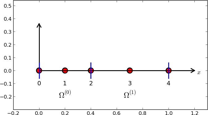
Example: Same mesh, but \( u \) is piecewise constant in each cell (P0 element).
Same vertices and cells, but
dof_map = [[0], [1]]
May think of one node in the middle of each element.
cells, vertices, and dof_map.
# Use modified fe_approx1D module
from fe_approx1D_numint import *

x = sp.Symbol('x')
f = x*(1 - x)

N_e = 10
# Create mesh with P3 (cubic) elements
vertices, cells, dof_map = mesh_uniform(N_e, d=3, Omega=[0,1])

# Create basis functions on the mesh
phi = [basis(len(dof_map[e])-1) for e in range(N_e)]

# Create linear system and solve it
A, b = assemble(vertices, cells, dof_map, phi, f)
c = np.linalg.solve(A, b)

# Make very fine mesh and sample u(x) on this mesh for plotting
x_u, u = u_glob(c, vertices, cells, dof_map,
                resolution_per_element=51)
plot(x_u, u)
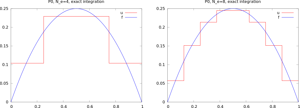
The approximate function automates the steps in the previous slide:
from fe_approx1D_numint import *
x=sp.Symbol("x")
for N_e in 4, 8:
    approximate(x*(1-x), d=0, N_e=N_e, Omega=[0,1])
$$ L^2 \hbox{ error: }\quad ||e||_{L^2} =
\left(\int_{\Omega} e^2 dx\right)^{1/2}$$
Accurate approximation of the integral:
u_glob, returns x and u)
$$ \int_\Omega g(x) dx \approx \sum_{j=0}^{n-1} \half(g(x_j) +
g(x_{j+1}))(x_{j+1}-x_j)$$
# Given c, compute x and u values on a very fine mesh
x, u = u_glob(c, vertices, cells, dof_map,
              resolution_per_element=101)
# Compute the error on the very fine mesh
e = f(x) - u
e2 = e**2
# Vectorized Trapezoidal rule
E = np.sqrt(0.5*np.sum((e2[:-1] + e2[1:])*(x[1:] - x[:-1]))
Theory and experiments show that the least squares or projection/Galerkin method in combination with Pd elements of equal length \( h \) has an error
$$
\begin{equation}
||e||_{L^2} = Ch^{d+1}
\tag{28}
\end{equation}
$$
where \( C \) depends on \( f \), but not on \( h \) or \( d \).
Consider a reference cell \( [-1,1] \). We introduce two nodes, \( X=-1 \) and \( X=1 \). The degrees of freedom are
4 constraints on \( \refphi_r \) (1 for dof \( r \), 0 for all others):
This gives 4 linear, coupled equations for each \( \refphi_r \) to determine the 4 coefficients in the cubic polynomial
$$
\begin{align}
\refphi_0(X) &= 1 - \frac{3}{4}(X+1)^2 + \frac{1}{4}(X+1)^3\\
\refphi_1(X) &= -(X+1)(1 - \half(X+1))^2\\
\refphi_2(X) &= \frac{3}{4}(X+1)^2 - \half(X+1)^3\\
\refphi_3(X) &= -\half(X+1)(\half(X+1)^2 - (X+1))\\
\end{align}
$$
Common form of a numerical integration rule:
$$
\begin{equation}
\int_{-1}^{1} g(X)dX \approx \sum_{j=0}^M w_jg(\bar X_j),
\end{equation}
$$
where
Different rules correspond to different choices of points and weights
Simplest possibility: the Midpoint rule,
$$
\begin{equation}
\int_{-1}^{1} g(X)dX \approx 2g(0),\quad \bar X_0=0,\ w_0=2,
\end{equation}
$$
Exact for linear integrands
The Trapezoidal rule:
$$
\begin{equation}
\int_{-1}^{1} g(X)dX \approx g(-1) + g(1),\quad \bar X_0=-1,\ \bar X_1=1,\ w_0=w_1=1,
\tag{29}
\end{equation}
$$
Simpson's rule:
$$
\begin{equation}
\int_{-1}^{1} g(X)dX \approx \frac{1}{3}\left(g(-1) + 4g(0)
+ g(1)\right),
\end{equation}
$$
where
$$
\begin{equation}
\bar X_0=-1,\ \bar X_1=0,\ \bar X_2=1,\ w_0=w_2=\frac{1}{3},\ w_1=\frac{4}{3}
\end{equation}
$$
$$
\begin{align}
M=1&:\quad \bar X_0=-\frac{1}{\sqrt{3}},\
\bar X_1=\frac{1}{\sqrt{3}},\ w_0=w_1=1\\
M=2&:\quad \bar X_0=-\sqrt{\frac{3}{{5}}},\ \bar X_0=0,\
\bar X_2= \sqrt{\frac{3}{{5}}},\ w_0=w_2=\frac{5}{9},\ w_1=\frac{8}{9}
\end{align}
$$
See numint.py for a large collection of Gauss-Legendre rules.
Inner product in 2D:
$$
\begin{equation}
(f,g) = \int_\Omega f(x,y)g(x,y) dx dy
\end{equation}
$$
Least squares and project/Galerkin lead to a linear system
$$
\begin{align*}
\sum_{j\in\If} A_{i,j}c_j &= b_i,\quad i\in\If\\
A_{i,j} &= (\baspsi_i,\baspsi_j)\\
b_i &= (f,\baspsi_i)
\end{align*}
$$
Challenge: How to construct 2D basis functions \( \baspsi_i(x,y) \)?
Use a 1D basis for \( x \) variation and a similar for \( y \) variation:
$$
\begin{align}
V_x &= \mbox{span}\{ \hat\baspsi_0(x),\ldots,\hat\baspsi_{N_x}(x)\}
\tag{30}\\
V_y &= \mbox{span}\{ \hat\baspsi_0(y),\ldots,\hat\baspsi_{N_y}(y)\}
\tag{31}
\end{align}
$$
The 2D vector space can be defined as a tensor product \( V = V_x\otimes V_y \) with basis functions
$$
\baspsi_{p,q}(x,y) = \hat\baspsi_p(x)\hat\baspsi_q(y)
\quad p\in\Ix,q\in\Iy\tp
$$
Given two vectors \( a=(a_0,\ldots,a_M) \) and \( b=(b_0,\ldots,b_N) \) their outer tensor product, also called the dyadic product, is \( p=a\otimes b \), defined through
$$ p_{i,j}=a_ib_j,\quad i=0,\ldots,M,\ j=0,\ldots,N\tp$$
Note: \( p \) has two indices (as a matrix or two-dimensional array)
Example: 2D basis as tensor product of 1D spaces,
$$ \baspsi_{p,q}(x,y) = \hat\baspsi_p(x)\hat\baspsi_q(y),
\quad p\in\Ix,q\in\Iy$$
The 2D basis can employ a double index and double sum:
$$ u = \sum_{p\in\Ix}\sum_{q\in\Iy} c_{p,q}\baspsi_{p,q}(x,y)
$$
Or just a single index:
$$ u = \sum_{j\in\If} c_j\baspsi_j(x,y)$$
with
$$
\baspsi_i(x,y) = \hat\baspsi_p(x)\hat\baspsi_q(y),
\quad i=p N_y + q\hbox{ or } i=q N_x + p
$$
In 1D we use the basis
$$ \{ 1, x \} $$
2D tensor product (all combinations):
$$ \baspsi_{0,0}=1,\quad \baspsi_{1,0}=x, \quad \baspsi_{0,1}=y,
\quad \baspsi_{1,1}=xy
$$
or with a single index:
$$ \baspsi_0=1,\quad \baspsi_1=x, \quad \baspsi_2=y,\quad\baspsi_3 =xy
$$
See notes for details of a hand-calculation.
Quadratic \( f(x,y) = (1+x^2)(1+2y^2) \) (left), bilinear \( u \) (right):

Very small modification of approx1D.py:
Omega = [[0, L_x], [0, L_y]]
import sympy as sp

integrand = psi[i]*psi[j]
I = sp.integrate(integrand,
                 (x, Omega[0][0], Omega[0][1]),
                 (y, Omega[1][0], Omega[1][1]))

# Fall back on numerical integration if symbolic integration
# was unsuccessful
if isinstance(I, sp.Integral):
    integrand = sp.lambdify([x,y], integrand)
    I = sp.mpmath.quad(integrand,
                       [Omega[0][0], Omega[0][1]],
                       [Omega[1][0], Omega[1][1]])
Tensor product of 1D "Taylor-style" polynomials \( x^i \):
def taylor(x, y, Nx, Ny):
    return [x**i*y**j for i in range(Nx+1) for j in range(Ny+1)]
Tensor product of 1D sine functions \( \sin((i+1)\pi x) \):
def sines(x, y, Nx, Ny):
    return [sp.sin(sp.pi*(i+1)*x)*sp.sin(sp.pi*(j+1)*y)
            for i in range(Nx+1) for j in range(Ny+1)]
Complete code in approx2D.py
\( f(x,y) = (1+x^2)(1+2y^2) \)
>>> from approx2D import *
>>> f = (1+x**2)*(1+2*y**2)
>>> psi = taylor(x, y, 1, 1)
>>> Omega = [[0, 2], [0, 2]]
>>> u, c = least_squares(f, psi, Omega)
>>> print u
8*x*y - 2*x/3 + 4*y/3 - 1/9
>>> print sp.expand(f)
2*x**2*y**2 + x**2 + 2*y**2 + 1
Add higher powers to the basis such that \( f\in V \):
>>> psi = taylor(x, y, 2, 2)
>>> u, c = least_squares(f, psi, Omega)
>>> print u
2*x**2*y**2 + x**2 + 2*y**2 + 1
>>> print u-f
0
Expected: \( u=f \) when \( f\in V \)
Key idea:
$$ V = V_x\otimes V_y\otimes V_z$$
$$
\begin{align*}
a^{(q)} &= (a^{(q)}_0,\ldots,a^{(q)}_{N_q}),\quad q=0,\ldots,m\\
p &= a^{(0)}\otimes\cdots\otimes a^{(m)}\\
p_{i_0,i_1,\ldots,i_m} &= a^{(0)}_{i_1}a^{(1)}_{i_1}\cdots a^{(m)}_{i_m}
\end{align*}
$$
$$
\begin{align*}
\baspsi_{p,q,r}(x,y,z) &= \hat\baspsi_p(x)\hat\baspsi_q(y)\hat\baspsi_r(z)\\
u(x,y,z) &= \sum_{p\in\Ix}\sum_{q\in\Iy}\sum_{r\in\Iz} c_{p,q,r}
\baspsi_{p,q,r}(x,y,z)
\end{align*}
$$
The two great advantages of the finite element method:
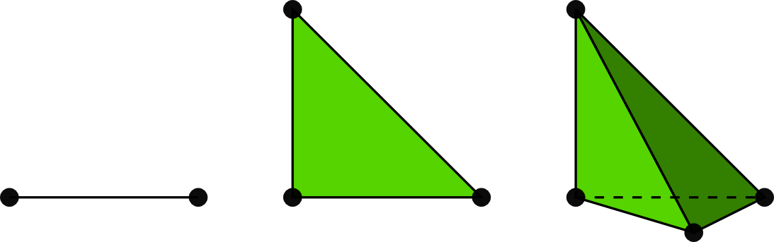
Finite elements in 1D: mostly for learning, insight, debugging
2D:
3D:


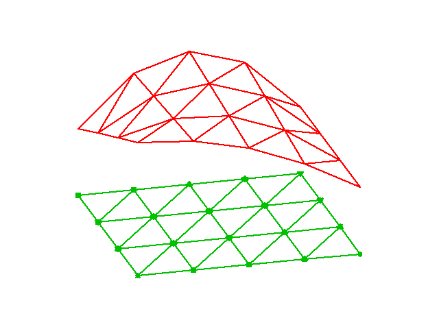
The P1 triangular 2D element: \( u \) is linear \( ax + by + c \) over each triangular cell
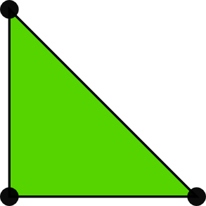
$$
\begin{align}
\refphi_0(X,Y) &= 1 - X - Y\\
\refphi_1(X,Y) &= X\\
\refphi_2(X,Y) &= Y
\end{align}
$$
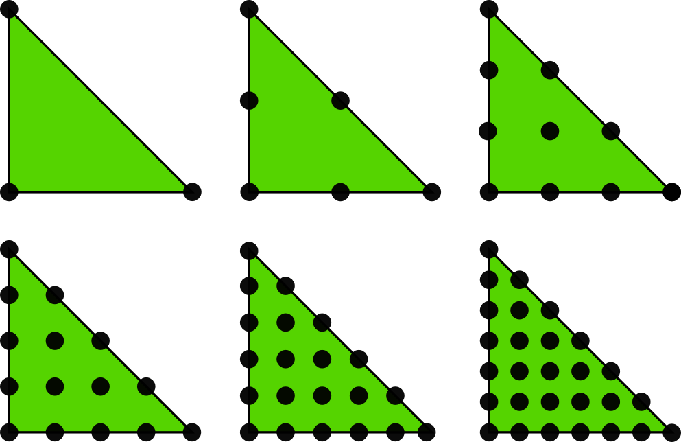
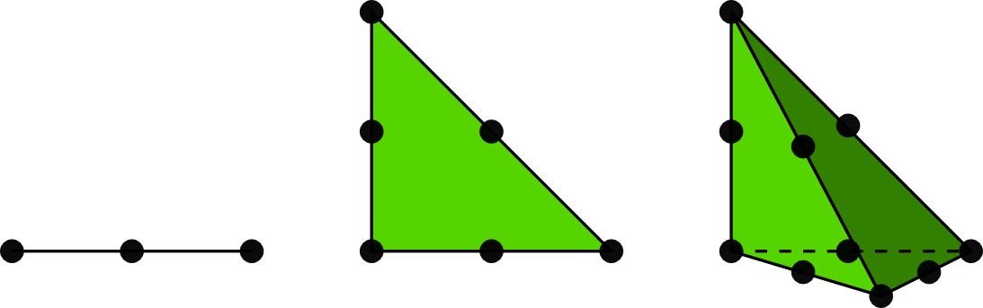
Higher-degree \( \refphi_r \) introduce more nodes (dof = node values)
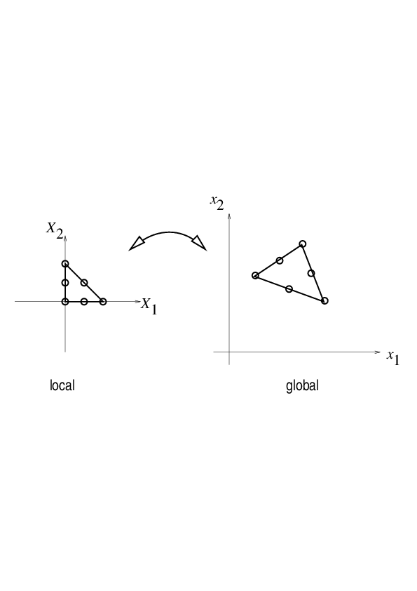
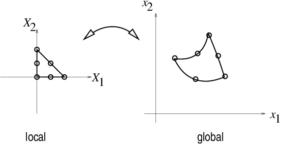
Mapping of local \( \X = (X,Y) \) coordinates in the reference cell to global, physical \( \x = (x,y) \) coordinates:
$$
\begin{equation}
\x = \sum_{r} \refphi_r^{(1)}(\X)\xdno{q(e,r)}
\tag{32}
\end{equation}
$$
where
This mapping preserves the straight/planar faces and edges.
Idea: Use the basis functions of the element (not only the P1 functions) to map the element
$$
\begin{equation}
\x = \sum_{r} \refphi_r(\X)\xdno{q(e,r)}
\tag{33}
\end{equation}
$$
Advantage: higher-order polynomial basis functions now map the reference cell to a curved triangle or tetrahedron.
Integrals must be transformed from \( \Omega^{(e)} \) (physical cell) to \( \tilde\Omega^r \) (reference cell):
$$
\begin{align}
\int_{\Omega^{(e)}}\basphi_i (\x) \basphi_j (\x) \dx &=
\int_{\tilde\Omega^r} \refphi_i (\X) \refphi_j (\X)
\det J\, \dX\\
\int_{\Omega^{(e)}}\basphi_i (\x) f(\x) \dx &=
\int_{\tilde\Omega^r} \refphi_i (\X) f(\x(\X)) \det J\, \dX
\end{align}
$$
where \( \dx = dx dy \) or \( \dx = dxdydz \) and \( \det J \) is the determinant of the
Jacobian of the mapping \( \x(\X) \).
$$
\begin{equation}
J = \left[\begin{array}{cc}
\frac{\partial x}{\partial X} & \frac{\partial x}{\partial Y}\\
\frac{\partial y}{\partial X} & \frac{\partial y}{\partial Y}
\end{array}\right], \quad
\det J = \frac{\partial x}{\partial X}\frac{\partial y}{\partial Y}
- \frac{\partial x}{\partial Y}\frac{\partial y}{\partial X}
\tag{34}
\end{equation}
$$
Affine mapping (32): \( \det J=2\Delta \), \( \Delta = \hbox{cell volume} \)
!slide
Our aim is to extend the ideas for approximating \( f \) by \( u \), or solving
$$ u = f $$
to real differential equations like[[[
$$ -u'' + bu = f,\quad u(0)=1,\ u'(L)=D $$
Three methods are addressed:
Method 2 will be totally dominating!
$$
\begin{equation}
\mathcal{L}(u) = 0,\quad x\in\Omega \end{equation}
$$
Examples (1D problems):
$$
\begin{align}
\mathcal{L}(u) &= \frac{d^2u}{dx^2} - f(x),
\tag{35}\\
\mathcal{L}(u) &= \frac{d}{dx}\left(\dfc(x)\frac{du}{dx}\right) + f(x),
\tag{36}\\
\mathcal{L}(u) &= \frac{d}{dx}\left(\dfc(u)\frac{du}{dx}\right) - au + f(x),
\tag{37}\\
\mathcal{L}(u) &= \frac{d}{dx}\left(\dfc(u)\frac{du}{dx}\right) + f(u,x)
\tag{38}
\end{align}
$$
$$
\begin{equation}
{\cal B}_0(u)=0,\ x=0,\quad {\cal B}_1(u)=0,\ x=L
\end{equation}
$$
Examples:
$$
\begin{align}
\mathcal{B}_i(u) &= u - g,\quad &\hbox{Dirichlet condition}\\
\mathcal{B}_i(u) &= -\dfc \frac{du}{dx} - g,\quad &\hbox{Neumann condition}\\
\mathcal{B}_i(u) &= -\dfc \frac{du}{dx} - h(u-g),\quad &\hbox{Robin condition}
\end{align}
$$
Much is similar to approximating a function (solving \( u=f \)), but two new topics are needed:
Inserting \( u=\sum_jc_j\baspsi_j \) in \( \mathcal{L}=0 \) gives a residual
$$
\begin{equation}
R = \mathcal{L}(u) = \mathcal{L}(\sum_j c_j \baspsi_j) \neq 0
\end{equation}
$$
Goal: minimize \( R \) wrt \( \sequencei{c} \) (and hope it makes a small \( e \) too)
$$ R=R(c_0,\ldots,c_N; x)$$
Idea: minimize
$$
\begin{equation}
E = ||R||^2 = (R,R) = \int_{\Omega} R^2 dx
\end{equation}
$$
Minimization wrt \( \sequencei{c} \) implies
$$
\begin{equation}
\frac{\partial E}{\partial c_i} =
\int_{\Omega} 2R\frac{\partial R}{\partial c_i} dx = 0\quad
\Leftrightarrow\quad (R,\frac{\partial R}{\partial c_i})=0,\quad
i\in\If
\tag{39}
\end{equation}
$$
\( N+1 \) equations for \( N+1 \) unknowns \( \sequencei{c} \)
Idea: make \( R \) orthogonal to \( V \),
$$
\begin{equation}
(R,v)=0,\quad \forall v\in V
\tag{40}
\end{equation}
$$
This implies
$$
\begin{equation}
(R,\baspsi_i)=0,\quad i\in\If
\tag{41}
\end{equation}
$$
\( N+1 \) equations for \( N+1 \) unknowns \( \sequencei{c} \)
Generalization of the Galerkin method: demand \( R \) orthogonal to some space \( W \), possibly \( W\neq V \):
$$
\begin{equation}
(R,v)=0,\quad \forall v\in W
\tag{42}
\end{equation}
$$
If \( \{w_0,\ldots,w_N\} \) is a basis for \( W \):
$$
\begin{equation}
(R,w_i)=0,\quad i\in\If
\tag{43}
\end{equation}
$$
Idea: demand \( R=0 \) at \( N+1 \) points
$$
\begin{equation}
R(\xno{i}; c_0,\ldots,c_N)=0,\quad i\in\If
\tag{44}
\end{equation}
$$
Note: The collocation method is a weighted residual method with delta functions as weights
$$ 0 = \int_\Omega R(x;c_0,\ldots,c_N)
\delta(x-\xno{i})\dx = R(\xno{i}; c_0,\ldots,c_N)$$
$$
\begin{equation}
\hbox{property of } \delta(x):\quad
\int_{\Omega} f(x)\delta (x-\xno{i}) dx = f(\xno{i}),\quad \xno{i}\in\Omega
\tag{45}
\end{equation}
$$
$$
\begin{equation}
-u''(x) = f(x),\quad x\in\Omega=[0,L],\quad u(0)=0,\ u(L)=0
\tag{46}
\end{equation}
$$
Basis functions:
$$
\begin{equation}
\baspsi_i(x) = \sinL{i},\quad i\in\If
\tag{47}
\end{equation}
$$
The residual:
$$
\begin{align}
R(x;c_0,\ldots,c_N) &= u''(x) + f(x),\nonumber\\
&= \frac{d^2}{dx^2}\left(\sum_{j\in\If} c_j\baspsi_j(x)\right)
+ f(x),\nonumber\\
&= -\sum_{j\in\If} c_j\baspsi_j''(x) + f(x)
\tag{48}
\end{align}
$$
Since \( u(0)=u(L)=0 \) we must ensure that all \( \baspsi_i(0)=\baspsi_i(L)=0 \). Then
$$ u(0) = \sum_jc_j\baspsi_j(0) = 0,\quad u(L) = \sum_jc_j\baspsi_j(L) $$
$$
(R,\frac{\partial R}{\partial c_i}) = 0,\quad i\in\If
$$
$$
\begin{equation}
\frac{\partial R}{\partial c_i} =
\frac{\partial}{\partial c_i}
\left(\sum_{j\in\If} c_j\baspsi_j''(x) + f(x)\right)
= \baspsi_i''(x) \end{equation}
$$
Because:
$$
\frac{\partial}{\partial c_i}\left(c_0\baspsi_0'' + c_1\baspsi_1'' + \cdots +
c_{i-1}\baspsi_{i-1}'' + \color{blue}{c_i\baspsi_{i}''} + c_{i+1}\baspsi_{i+1}''
+ \cdots + c_N\baspsi_N'' \right) = \baspsi_{i}''
$$
$$
\begin{equation}
(\sum_j c_j \baspsi_j'' + f,\baspsi_i'')=0,\quad i\in\If
\end{equation}
$$
Rearrangement:
$$
\begin{equation}
\sum_{j\in\If}(\baspsi_i'',\baspsi_j'')c_j = -(f,\baspsi_i''),\quad i\in\If \end{equation}
$$
This is a linear system
$$
\begin{equation*} \sum_{j\in\If}A_{i,j}c_j = b_i,\quad i\in\If
\end{equation*}
$$
with
$$
\begin{align}
A_{i,j} &= (\baspsi_i'',\baspsi_j'')\nonumber\\
& = \pi^4(i+1)^2(j+1)^2L^{-4}\int_0^L \sinL{i}\sinL{j}\, dx\nonumber\\
&= \left\lbrace
\begin{array}{ll} {1\over2}L^{-3}\pi^4(i+1)^4 & i=j \\ 0, & i\neq j
\end{array}\right.
\\
b_i &= -(f,\baspsi_i'') = (i+1)^2\pi^2L^{-2}\int_0^Lf(x)\sinL{i}\, dx
\end{align}
$$
Useful property:
$$
\begin{equation}
\int\limits_0^L \sinL{i}\sinL{j}\, dx = \delta_{ij},\quad
\quad\delta_{ij} = \left\lbrace
\begin{array}{ll} \half L & i=j \\ 0, & i\neq j
\end{array}\right.
\end{equation}
$$
\( \Rightarrow\ (\baspsi_i'',\baspsi_j'') = \delta_{ij} \), i.e., diagonal \( A_{i,j} \), and we can easily solve for \( c_i \):
$$
\begin{equation}
c_i = \frac{2L}{\pi^2(i+1)^2}\int_0^Lf(x)\sinL{i}\, dx
\tag{49}
\end{equation}
$$
Let's sympy do the work (\( f(x)=2 \)):
from sympy import *
import sys

i, j = symbols('i j', integer=True)
x, L = symbols('x L')
f = 2
a = 2*L/(pi**2*(i+1)**2)
c_i = a*integrate(f*sin((i+1)*pi*x/L), (x, 0, L))
c_i = simplify(c_i)
print c_i
$$
\begin{equation}
c_i = 4 \frac{L^{2} \left(\left(-1\right)^{i} + 1\right)}{\pi^{3}
\left(i^{3} + 3 i^{2} + 3 i + 1\right)},\quad
u(x) = \sum_{k=0}^{N/2} \frac{8L^2}{\pi^3(2k+1)^3}\sinL{2k}\tp
\end{equation}
$$
Fast decay: \( c_2 = c_0/27 \), \( c_4=c_0/125 \) - only one term might be good enough:
$$
\begin{equation*} u(x) \approx \frac{8L^2}{\pi^3}\sin\left(\pi\frac{x}{L}\right)\tp \end{equation*}
$$
\( R=u''+f \):
$$
\begin{equation*}
(u''+f,v)=0,\quad \forall v\in V,
\end{equation*}
$$
or
$$
\begin{equation}
(u'',v) = -(f,v),\quad\forall v\in V \end{equation}
$$
This is a variational formulation of the differential equation problem.
\( \forall v\in V \) means for all basis functions:
$$
\begin{equation}
(\sum_{j\in\If} c_j\baspsi_j'', \baspsi_i)=-(f,\baspsi_i),\quad i\in\If \end{equation}
$$
Since \( \baspsi_i''\propto \baspsi_i \), Galerkin's method gives the same linear system and the same solution as the least squares method (in this particular example).
\( R=0 \) (i.e.,the differential equation) must be satisfied at \( N+1 \) points:
$$
\begin{equation}
-\sum_{j\in\If} c_j\baspsi_j''(\xno{i}) = f(\xno{i}),\quad i\in\If
\end{equation}
$$
This is a linear system \( \sum_j A_{i,j}=b_i \) with entries
$$
\begin{equation*} A_{i,j}=-\baspsi_j''(\xno{i})=
(j+1)^2\pi^2L^{-2}\sin\left((j+1)\pi \frac{x_i}{L}\right),
\quad b_i=2
\end{equation*}
$$
Choose: \( N=0 \), \( x_0=L/2 \)
$$ c_0=2L^2/\pi^2 $$
Second-order derivatives will hereafter be integrated by parts
$$
\begin{align}
\int_0^L u''(x)v(x) dx &= - \int_0^Lu'(x)v'(x)dx
+ [vu']_0^L\nonumber\\
&= - \int_0^Lu'(x)v'(x) dx
+ u'(L)v(L) - u'(0)v(0)
\tag{50}
\end{align}
$$
Motivation:
Dirichlet conditions: \( u(0)=C \) and \( u(L)=D \). Choose for example
$$ B(x) = \frac{1}{L}(C(L-x) + Dx):\qquad B(0)=C,\ B(L)=D $$
$$
\begin{equation}
u(x) = B(x) + \sum_{j\in\If} c_j\baspsi_j(x),
\tag{51}
\end{equation}
$$
$$ u(0) = B(0)= C,\quad u(L) = B(L) = D $$
Dirichlet condition: \( u(L)=D \). Choose for example
$$ B(x) = D:\qquad B(L)=D $$
$$
\begin{equation}
u(x) = B(x) + \sum_{j\in\If} c_j\baspsi_j(x),
\tag{51}
\end{equation}
$$
$$ u(L) = B(L) = D $$
The finite element literature (and much FEniCS documentation) applies an abstract notation for the variational formulation:
$$ a(u,v) = L(v)\quad \forall v\in V $$
$$ -u''=f, \quad u'(0)=C,\ u(L)=D,\quad u=D + \sum_jc_j\baspsi_j$$
Variational formulation:
$$
\int_{\Omega} u' v'dx = \int_{\Omega} fvdx\quad - v(0)C
\hbox{or}\quad (u',v') = (f,v) - v(0)C
\quad\forall v\in V
$$
Abstract formulation: finn \( (u-B)\in V \) such that
$$ a(u,v) = L(v)\quad \forall v\in V$$
We identify
$$ a(u,v) = (u',v'),\quad L(v) = (f,v) -v(0)C $$
Linear form means
$$ L(\alpha_1 v_1 + \alpha_2 v_2)
=\alpha_1 L(v_1) + \alpha_2 L(v_2),
$$
Bilinear form means
$$
\begin{align*}
a(\alpha_1 u_1 + \alpha_2 u_2, v) &= \alpha_1 a(u_1,v) + \alpha_2 a(u_2, v),
\\
a(u, \alpha_1 v_1 + \alpha_2 v_2) &= \alpha_1 a(u,v_1) + \alpha_2 a(u, v_2)
\end{align*}
$$
In nonlinear problems: Find \( (u-B)\in V \) such that \( F(u;v)=0\ \forall v\in V \)
$$ a(u,v) = L(v)\quad \forall v\in V\quad\Leftrightarrow\quad
a(u,\baspsi_i) = L(\baspsi_i)\quad i\in\If$$
We can now derive the corresponding linear system once and for all:
$$ a(\sum_{j\in\If} c_j \baspsi_j,\baspsi_i)c_j = L(\baspsi_i)\quad i\in\If$$
Because of linearity,
$$ \sum_{j\in\If} \underbrace{a(\baspsi_j,\baspsi_i)}_{A_{i,j}}c_j =
\underbrace{L(\baspsi_i)}_{b_i}\quad i\in\If$$
$$ A_{i,j} = a(\baspsi_j,\baspsi_i),\quad
b_i = L(\baspsi_i) $$
If \( a(u,v)=a(v,u) \),
$$ a(u,v)=L(v)\quad\forall v\in V,$$
is equivalent to minimizing the functional
$$ F(v) = {\half}a(v,v) - L(v) $$
over all functions \( v\in V \). That is,
$$ F(u)\leq F(v)\quad \forall v\in V\tp $$
$$
\begin{equation}
-\frac{d}{dx}\left( \dfc(x)\frac{du}{dx}\right) = f(x),\quad x\in\Omega =[0,L],\
u(0)=C,\ u(L)=D
\end{equation}
$$
$$
u(x) = B(x) + \sum_{j\in\If} c_j\baspsi_i(x)
$$
$$ B(x) = C + \frac{1}{L}(D-C)x$$
$$ R = -\frac{d}{dx}\left( a\frac{du}{dx}\right) -f $$
Galerkin's method:
$$
(R, v) = 0,\quad \forall v\in V,
$$
or with integrals:
$$
\int_{\Omega} \left(\frac{d}{dx}\left( \dfc\frac{du}{dx}\right) -f\right)v \dx = 0,\quad \forall v\in V \tp
$$
Integration by parts:
$$ -\int_{\Omega} \frac{d}{dx}\left( \dfc(x)\frac{du}{dx}\right) v \dx
= \int_{\Omega} \dfc(x)\frac{du}{dx}\frac{dv}{dx}\dx -
\left[\dfc\frac{du}{dx}v\right]_0^L
\tp
$$
Boundary terms vanish since \( v(0)=v(L)=0 \)
Find \( (u-B)\in V \) such that
$$
\int_{\Omega} \dfc(x)\frac{du}{dx}\frac{dv}{dx}dx = \int_{\Omega} f(x)vdx,\quad
\forall v\in V,
$$
Compact notation:
$$ \underbrace{(\dfc u',v')}_{a(u,v)} = \underbrace{(f,v)}_{L(v)},
\quad \forall v\in V $$
With
$$ a(u,v) = (\dfc u', v),\quad L(v) = (f,v) $$
we can just use the formula for the linear system:
$$
\begin{align*}
A_{i,j} &= a(\baspsi_j,\baspsi_i) = (\dfc \baspsi_j', \baspsi_i')
= \int_\Omega \dfc \baspsi_j' \baspsi_i'\dx =
\int_\Omega \baspsi_i' \dfc \baspsi_j'\dx = a(\baspsi_i,\baspsi_j) = A_{j,i}\\
b_i &= (f,\baspsi_i) = \int_\Omega f\baspsi_i\dx
\end{align*}
$$
\( v=\baspsi_i \) and \( u=B + \sum_jc_j\baspsi_j \):
$$
(\dfc B' + \dfc \sum_{j\in\If} c_j \baspsi_j', \baspsi_i') =
(f,\baspsi_i), \quad i\in\If \tp
$$
Reorder to form linear system:
$$ \sum_{j\in\If} (\dfc\baspsi_j', \baspsi_i')c_j =
(f,\baspsi_i) + (a(D-C)L^{-1}, \baspsi_i'), \quad i\in\If
\tp
$$
This is \( \sum_j A_{i,j}c_j=b_i \) with
$$
\begin{align*}
A_{i,j} &= (a\baspsi_j', \baspsi_i') = \int_{\Omega} \dfc(x)\baspsi_j'(x)
\baspsi_i'(x)\dx\\
b_i &= (f,\baspsi_i) + (a(D-C)L^{-1},\baspsi_i')=
\int_{\Omega} \left(f(x)\baspsi_i(x) + \dfc(x)\frac{D-C}{L}\baspsi_i'(x)\right) \dx
\end{align*}
$$
$$
\begin{equation}
-u''(x) + bu'(x) = f(x),\quad x\in\Omega =[0,L],\
u(0)=C,\ u'(L)=E
\end{equation}
$$
New features:
Initial steps:
$$ u = C + \sum_{j\in\If} c_j \baspsi_i(x)$$
Galerkin's method: multiply by \( v \), integrate over \( \Omega \), integrate by parts.
$$ (-u'' + bu' - f, v) = 0,\quad\forall v\in V$$
$$ (u',v') + (bu',v) = (f,v) + [u' v]_0^L, \quad\forall v\in V$$
Now, \( [u' v]_0^L = u'(L)v(L) = E v(L) \) because \( v(0)=0 \) and \( u'(L)=E \):
$$ (u'v') + (bu',v) = (f,v) + Ev(L), \quad\forall v\in V$$
$$ (u'v') + (bu',v) = (f,v) + Ev(L), \quad\forall v\in V,$$
Important:
Abstract notation:
$$ a(u,v)=L(v)\quad\forall v\in V$$
Here:
$$
\begin{align*}
a(u,v)&=(u',v') + (bu',v)\\
L(v)&= (f,v) + E v(L)
\end{align*}
$$
Insert \( u=C+\sum_jc_j\baspsi_j \) and \( v=\baspsi_i \):
$$
\sum_{j\in\If}
\underbrace{((\baspsi_j',\baspsi_i') + (b\baspsi_j',\baspsi_i))}_{A_{i,j}}
c_j =
\underbrace{(f,\baspsi_i) + E \baspsi_i(L)}_{b_i}
$$
Observation: \( A_{i,j} \) is not symmetric because of the term
$$
(b\baspsi_j',\baspsi_i)=\int_{\Omega} b\baspsi_j'\baspsi_i dx
\neq \int_{\Omega} b \baspsi_i' \baspsi_jdx = (\baspsi_i',b\baspsi_j)
$$
$$ (u',v') + (bu',v) = (f,v) + u'(L)v(L) - u'(0)v(0)$$
Problem:
$$
\begin{equation}
-(\dfc(u)u')' = f(u),\quad x\in [0,L],\ u(0)=0,\ u'(L)=E
\end{equation}
$$
Galerkin: multiply by \( v \), integrate, integrate by parts
$$ \int_0^L \dfc(u)\frac{du}{dx}\frac{dv}{dx}\dx =
\int_0^L f(u)v\dx + [\dfc(u)vu']_0^L\quad\forall v\in V
$$
$$ \int_0^L \dfc(u)\frac{du}{dx}\frac{dv}{dx}v\dx =
\int_0^L f(u)v\dx + \dfc(u(L))v(L)E\quad\forall v\in V
$$
or
$$ (\dfc(u)u', v') = (f(u),v) + \dfc(u(L))v(L)E\quad\forall v\in V
$$
$$
\begin{equation*}
-u''(x)=f(x),\quad x\in \Omega=[0,1],\quad u'(0)=C,\ u(1)=D
\end{equation*}
$$
$$ A_{i,j} = (\baspsi_j',\baspsi_i') = \int_{0}^1 \baspsi_i'(x)\baspsi_j'(x)dx
= \int_0^1 (i+1)(j+1)(1-x)^{i+j} dx,
$$
Choose \( f(x)=2 \):
$$
\begin{align*}
b_i &= (2,\baspsi_i) - (D,\baspsi_i') -C\baspsi_i(0)\\
&= \int_0^1 \left( 2(1-x)^{i+1} - D(i+1)(1-x)^i\right)dx -C\baspsi_i(0)
\end{align*}
$$
Can easily do the integrals with sympy. \( N=1 \):
$$
\begin{equation*}
\left(\begin{array}{cc}
1 & 1\\
1 & 4/3
\end{array}\right)
\left(\begin{array}{c}
c_0\\
c_1
\end{array}\right)
=
\left(\begin{array}{c}
-C+D+1\\
2/3 -C + D
\end{array}\right)
\end{equation*}
$$
$$ c_0=-C+D+2, \quad c_1=-1,$$
$$ u(x) = 1 -x^2 + D + C(x-1)\quad\hbox{(exact solution)} $$
Assume that apart from boundary conditions, \( \uex \) lies in the same space \( V \) as where we seek \( u \):
$$
\begin{align*}
u &= B + F,\quad F\in V
a(B+F, v) &= L(v)\quad\forall v\in V
\uex & = B + E,\quad E\in V
a(B+E, v) &= L(v)\quad\forall v\in V
\end{align*}
$$
Subtract: \( a(F-E,v)=0\ \Rightarrow\ E=F \) and \( u = \uex \)
Tasks:
$$ -u''(x) = 2,\quad x\in (0,L),\ u(0)=u(L)=0,$$
Variational formulation:
$$ (u',v') = (2,v)\quad\forall v\in V $$
Since \( u(0)=0 \) and \( u(L)=0 \), we must force
$$ v(0)=v(L)=0,\quad \baspsi_i(0)=\baspsi_i(L)=0$$
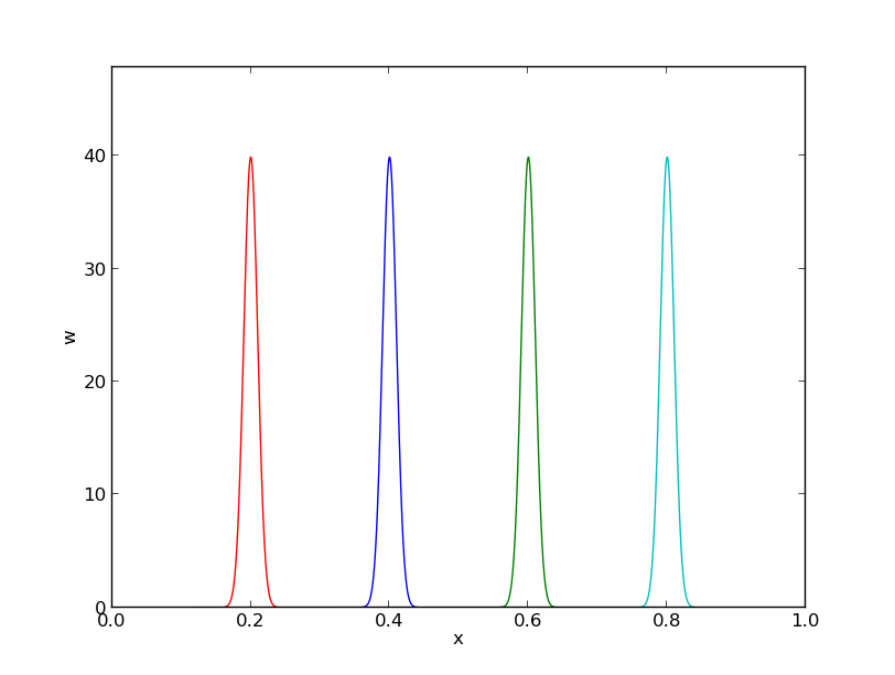
Use finite element basis, but exclude \( \basphi_0 \) and \( \basphi_{N_n} \) since these are not 0 on the boundary:
$$ \baspsi_i=\basphi_{i+1},\quad i=0,\ldots,N=N_n-2$$
Introduce index mapping \( \nu(j) \): \( \baspsi_i = \basphi_{\nu(i)} \)
$$ u = \sum_{j\in\If}c_j\basphi_{\nu(i)},\quad i=0,\ldots,N,\quad \nu(j) = j+1$$
Irregular numbering: more complicated \( \nu(j) \) table
$$
\begin{equation*}
A_{i,j}=\int_0^L\basphi_{i+1}'(x)\basphi_{j+1}'(x) dx,\quad
b_i=\int_0^L2\basphi_{i+1}(x) dx
\end{equation*}
$$
Many will prefer to change indices to obtain a \( \basphi_i'\basphi_j' \) product: \( i+1\rightarrow i \), \( j+1\rightarrow j \)
$$
\begin{equation*}
A_{i-1,j-1}=\int_0^L\basphi_{i}'(x)\basphi_{j}'(x) \dx,\quad
b_{i-1}=\int_0^L2\basphi_{i}(x) \dx
\end{equation*}
$$
$$ \basphi_i = \pm h^{-1} $$
$$ A_{i-1,i-1} = h^{-2}2h = 2h^{-1},\quad
A_{i-1,i-2} = h^{-1}(-h^{-1})h = -h^{-1},\quad A_{i-1,i}=A_{i-1,i-2}$$
$$ b_{i-1} = 2({\half}h + {\half}h) = 2h$$
$$
\begin{equation}
\frac{1}{h}\left(
\begin{array}{ccccccccc}
2 & -1 & 0
&\cdots &
\cdots & \cdots & \cdots &
\cdots & 0 \\
-1 & 2 & -1 & \ddots & & & & & \vdots \\
0 & -1 & 2 & -1 &
\ddots & & & & \vdots \\
\vdots & \ddots & & \ddots & \ddots & 0 & & & \vdots \\
\vdots & & \ddots & \ddots & \ddots & \ddots & \ddots & & \vdots \\
\vdots & & & 0 & -1 & 2 & -1 & \ddots & \vdots \\
\vdots & & & & \ddots & \ddots & \ddots &\ddots & 0 \\
\vdots & & & & &\ddots & \ddots &\ddots & -1 \\
0 &\cdots & \cdots &\cdots & \cdots & \cdots & 0 & -1 & 2
\end{array}
\right)
\left(
\begin{array}{c}
c_0 \\
\vdots\\
\vdots\\
\vdots \\
\vdots \\
\vdots \\
\vdots \\
\vdots\\
c_{N}
\end{array}
\right)
=
\left(
\begin{array}{c}
2h \\
\vdots\\
\vdots\\
\vdots \\
\vdots \\
\vdots \\
\vdots \\
\vdots\\
2h
\end{array}
\right)
\tag{53}
\end{equation}
$$
$$
\begin{equation}
-\frac{1}{h}u_{i-1} + \frac{2}{h}u_{i} - \frac{1}{h}u_{i+1} = 2h
\tag{54}
\end{equation}
$$
The standard finite difference method for \( -u''=2 \) is
$$ -\frac{1}{h^2}u_{i-1} + \frac{2}{h^2}u_{i} - \frac{1}{h^2}u_{i+1} = 2 $$
(Remains to study the equations involving boundary values)
$$
\begin{equation*}
A_{i-1,j-1}^{(e)}=\int_{\Omega^{(e)}} \basphi_i'(x)\basphi_j'(x) \dx
= \int_{-1}^1 \frac{d}{dx}\refphi_r(X)\frac{d}{dx}\refphi_s(X)
\frac{h}{2} \dX,
\end{equation*}
$$
$$ \refphi_0(X)=\half(1-X),\quad\refphi_1(X)=\half(1+X)$$
$$ \frac{d\refphi_0}{dX} = -\half,\quad \frac{d\refphi_1}{dX} = \half $$
From the chain rule
$$ \frac{d\refphi_r}{dx} = \frac{d\refphi_r}{dX}\frac{dX}{dx}
= \frac{2}{h}\frac{d\refphi_r}{dX}$$
$$
\begin{equation*}
A_{i-1,j-1}^{(e)}=\int_{\Omega^{(e)}} \basphi_i'(x)\basphi_j'(x) \dx
= \int_{-1}^1 \frac{2}{h}\frac{d\refphi_r}{dX}\frac{2}{h}\frac{d\refphi_s}{dX}
\frac{h}{2} \dX = \tilde A_{r,s}^{(e)}
\end{equation*}
$$
$$
\begin{equation*}
b_{i-1}^{(e)} = \int_{\Omega^{(e)}} 2\basphi_i(x) \dx =
\int_{-1}^12\refphi_r(X)\frac{h}{2} \dX = \tilde b_{r}^{(e)},
\quad i=q(e,r),\ r=0,1
\end{equation*}
$$
Must run through all \( r,s=0,1 \) and \( r=0,1 \) and compute each entry in the element matrix and vector:
$$
\begin{equation}
\tilde A^{(e)} =\frac{1}{h}\left(\begin{array}{rr}
1 & -1\\
-1 & 1
\end{array}\right),\quad
\tilde b^{(e)} = h\left(\begin{array}{c}
1\\
1
\end{array}\right)\tp
\tag{55}
\end{equation}
$$
Example:
$$ \tilde A^{(e)}_{0,1} =
\int_{-1}^1 \frac{2}{h}\frac{d\refphi_0}{dX}\frac{2}{h}\frac{d\refphi_1}{dX}
\frac{h}{2} \dX
= \frac{2}{h}(-\half)\frac{2}{h}\half\frac{h}{2} \int_{-1}^1\dX
= -\frac{1}{h}
$$
For \( e=0 \) and \( =N_e \):
$$
\tilde A^{(e)} =\frac{1}{h}\left(\begin{array}{r}
1
\end{array}\right),\quad
\tilde b^{(e)} = h\left(\begin{array}{c}
1
\end{array}\right)
$$
Only one degree of freedom ("node") in these cells (\( r=0 \) counts the only dof)
4 P1 elements:
vertices = [0, 0.5, 1, 1.5, 2]
cells = [[0, 1], [1, 2], [2, 3], [3, 4]]
dof_map = [[0], [0, 1], [1, 2], [2]]       # only 1 dof in elm 0, 3
Python code for the assembly algorithm:
# Ae[e][r,s]: element matrix, be[e][r]: element vector
# A[i,j]: coefficient matrix, b[i]: right-hand side

for e in range(len(Ae)):
    for r in range(Ae[e].shape[0]):
        for s in range(Ae[e].shape[1]):
            A[dof_map[e,r],dof_map[e,s]] += Ae[e][i,j]
        b[dof_map[e,r]] += be[e][i,j]
Result: same linear system as arose from computations in the physical domain
$$
\begin{equation}
B(x) = \sum_{j\in\Ifb} U_j\basphi_j(x)
\end{equation}
$$
Suppose we have a Dirichlet condition \( u(\xno{k})=U_k \), \( k\in\Ifb \):
$$
u(\xno{k}) = \sum_{j\in\Ifb} U_j\underbrace{\basphi_j(x)}_{\neq 0
\hbox{ only for }j=k} +
\sum_{j\in\If} c_j\underbrace{\basphi_{\nu(j)}(\xno{k})}_{=0,\ k\not\in\If}
= U_k $$
$$ -u''=2, \quad u(0)=C,\ u(L)=D $$
$$ \int_0^L u'v'\dx = \int_0^L2v\dx\quad\forall v\in V$$
$$ (u',v') = (2,v)\quad\forall v\in V$$
$$
\begin{equation}
B(x) = \sum_{j\in\Ifb} U_j\basphi_j(x)
\end{equation}
$$
Here \( \Ifb = \{0,N_n\} \), \( U_0=C \), \( U_{N_n}=D \),
$$ \baspsi_i = \basphi_{\nu(i)}, \quad \nu(i)=i+1,\quad i\in\If =
\{0,\ldots,N=N_n-2\} $$
$$
\begin{equation}
u(x) = C\basphi_0(x) + D\basphi_{N_n}(x)
+ \sum_{j\in\If}c_j\basphi_{\nu(j)}
\end{equation}
$$
Insert \( u = B + \sum_j c_j\baspsi_j \) in variational formulation:
$$ (u',v') = (2,v)\quad\Rightarrow\quad (\sum_jc_j\baspsi_j',\baspsi_i')
= (2-B',\baspsi_i)\quad \forall v\in V$$
$$
\begin{align*}
u(x) &= \underbrace{C\cdot\basphi_0 + D\basphi_{N_n}}_{B(x)}
+ \sum_{j\in\If} c_j\basphi_{j+1}\\
&= C\cdot\basphi_0 + D\basphi_{N_n} + c_0\basphi_1 + c_1\basphi_2 +\cdots
+ c_N\basphi_{N_n-1}
\end{align*}
$$
$$
A_{i-1,j-1} = \int_0^L \basphi_i'(x)\basphi_j'(x) \dx,\quad
b_{i-1} = \int_0^L (f(x) - C\basphi_{0}'(x) - D\basphi_{N_n}'(x))
\basphi_i(x) \dx
$$
for \( i,j = 1,\ldots,N+1=N_n-1 \).
New boundary terms from \( -\int B'\basphi_i\dx \): \( C/2 \) for \( i=1 \) and \( -D/2 \) for \( i=N_n-1 \)
From the last cell:
$$
\tilde b_0^{(N_e)} = \int_{-1}^1 \left(f - D\frac{2}{h}
\frac{d\refphi_1}{dX}\right)
\refphi_0\frac{h}{2} \dX
= (\frac{h}{2}(2 - D\frac{2}{h}\half)
\int_{-1}^1 \refphi_0 \dX = h - D/2
$$
From the first cell:
$$
\tilde b_0^{(0)} = \int_{-1}^1 \left(f - C\frac{2}{h}
\frac{d\refphi_0}{dX}\right)
\refphi_1\frac{h}{2} \dX
= (\frac{h}{2}(2 + C\frac{2}{h}\half)
\int_{-1}^1 \refphi_1 \dX = h + C/2\tp
$$
Method 2: always \( \baspsi_i = \basphi_i \) and
$$
\begin{equation}
u(x) = \sum_{j\in\If}c_j\basphi_j(x),\quad \If=\{0,\ldots,N=N_n\}
\tag{56}
\end{equation}
$$
$$ -u''=2,\quad u(0)=0,\ u(L)=D$$
Assemble as if there were no Dirichlet conditions:
$$
\begin{equation}
\frac{1}{h}\left(
\begin{array}{ccccccccc}
1 & -1 & 0
&\cdots &
\cdots & \cdots & \cdots &
\cdots & 0 \\
-1 & 2 & -1 & \ddots & & & & & \vdots \\
0 & -1 & 2 & -1 &
\ddots & & & & \vdots \\
\vdots & \ddots & & \ddots & \ddots & 0 & & & \vdots \\
\vdots & & \ddots & \ddots & \ddots & \ddots & \ddots & & \vdots \\
\vdots & & & 0 & -1 & 2 & -1 & \ddots & \vdots \\
\vdots & & & & \ddots & \ddots & \ddots &\ddots & 0 \\
\vdots & & & & &\ddots & \ddots &\ddots & -1 \\
0 &\cdots & \cdots &\cdots & \cdots & \cdots & 0 & -1 & 1
\end{array}
\right)
\left(
\begin{array}{c}
c_0 \\
\vdots\\
\vdots\\
\vdots \\
\vdots \\
\vdots \\
\vdots \\
\vdots\\
c_{N}
\end{array}
\right)
=
\left(
\begin{array}{c}
h \\
2h\\
\vdots\\
\vdots \\
\vdots \\
\vdots \\
\vdots \\
2h\\
h
\end{array}
\right)
\tag{57}
\end{equation}
$$
$$
\begin{equation}
\frac{1}{h}\left(
\begin{array}{ccccccccc}
h & 0 & 0
&\cdots &
\cdots & \cdots & \cdots &
\cdots & 0 \\
-1 & 2 & -1 & \ddots & & & & & \vdots \\
0 & -1 & 2 & -1 &
\ddots & & & & \vdots \\
\vdots & \ddots & & \ddots & \ddots & 0 & & & \vdots \\
\vdots & & \ddots & \ddots & \ddots & \ddots & \ddots & & \vdots \\
\vdots & & & 0 & -1 & 2 & -1 & \ddots & \vdots \\
\vdots & & & & \ddots & \ddots & \ddots &\ddots & 0 \\
\vdots & & & & &\ddots & \ddots &\ddots & -1 \\
0 &\cdots & \cdots &\cdots & \cdots & \cdots & 0 & 0 & h
\end{array}
\right)
\left(
\begin{array}{c}
c_0 \\
\vdots\\
\vdots\\
\vdots \\
\vdots \\
\vdots \\
\vdots \\
\vdots\\
c_{N}
\end{array}
\right)
=
\left(
\begin{array}{c}
0 \\
2h\\
\vdots\\
\vdots \\
\vdots \\
\vdots \\
\vdots \\
2h\\
D
\end{array}
\right)
\tag{58}
\end{equation}
$$
In cell 0 we know \( u \) for local node (degree of freedom) \( r=0 \). Replace the first cell equation by \( \tilde c_0 = 0 \):
$$
\begin{equation}
\tilde A^{(0)} =
A = \frac{1}{h}\left(\begin{array}{rr}
h & 0\\
-1 & 1
\end{array}\right),\quad
\tilde b^{(0)} = \left(\begin{array}{c}
0\\
h
\end{array}\right)
\tag{59}
\end{equation}
$$
In cell \( N_e \) we know \( u \) for local node \( r=1 \). Replace the last equation in the cell system by \( \tilde c_1=D \):
$$
\begin{equation}
\tilde A^{(N_e)} =
A = \frac{1}{h}\left(\begin{array}{rr}
1 & -1\\
0 & h
\end{array}\right),\quad
\tilde b^{(N_e)} = \left(\begin{array}{c}
h\\
D
\end{array}\right)
\tag{60}
\end{equation}
$$
Algorithm for incorporating \( c_i=U_i \) in a symmetric way:
$$
\begin{equation}
\frac{1}{h}\left(
\begin{array}{ccccccccc}
1 & 0 & 0
&\cdots &
\cdots & \cdots & \cdots &
\cdots & 0 \\
0 & 2 & -1 & \ddots & & & & & \vdots \\
0 & -1 & 2 & -1 &
\ddots & & & & \vdots \\
\vdots & \ddots & & \ddots & \ddots & 0 & & & \vdots \\
\vdots & & \ddots & \ddots & \ddots & \ddots & \ddots & & \vdots \\
\vdots & & & 0 & -1 & 2 & -1 & \ddots & \vdots \\
\vdots & & & & \ddots & \ddots & \ddots &\ddots & 0 \\
\vdots & & & & &\ddots & \ddots &\ddots & 0 \\
0 &\cdots & \cdots &\cdots & \cdots & \cdots & 0 & 0 & 1
\end{array}
\right)
\left(
\begin{array}{c}
c_0 \\
\vdots\\
\vdots\\
\vdots \\
\vdots \\
\vdots \\
\vdots \\
\vdots\\
c_{N}
\end{array}
\right)
=
\left(
\begin{array}{c}
0 \\
2h\\
\vdots\\
\vdots \\
\vdots \\
\vdots \\
\vdots \\
2h +D/h\\
D
\end{array}
\right)
\tag{61}
\end{equation}
$$
Symmetric modification applied to \( \tilde A^{(N_e)} \):
$$
\begin{equation}
\tilde A^{(N_e)} =
A = \frac{1}{h}\left(\begin{array}{rr}
1 & 0\\
0 & 1
\end{array}\right),\quad
\tilde b^{(N-1)} = \left(\begin{array}{c}
h + D/h\\
D
\end{array}\right)
\tag{62}
\end{equation}
$$
$$ -u''=f,\quad u'(0)=C,\ u(L)=D$$
Galerkin's method:
$$
\begin{equation*}
\int_0^L(u''(x)+f(x))\baspsi_i(x) dx = 0,\quad i\in\If
\end{equation*}
$$
Integration of \( u''\baspsi_i \) by parts:
$$
\begin{equation*}
\int_0^Lu'(x)\baspsi_i'(x) \dx -(u'(L)\baspsi_i(L) - u'(0)\baspsi_i(0)) -
\int_0^L f(x)\baspsi_i(x) \dx =0, \quad i\in\If
\end{equation*}
$$
$$
\begin{equation*}
\int_0^Lu'(x)\basphi_i'(x) dx =
\int_0^L f(x)\basphi_i(x) dx - C\basphi_i(0),\quad i\in\If
\end{equation*}
$$
$$
\begin{equation}
\sum_{j=0}^{N=N_n-1}\left(
\int_0^L \basphi_i'(x)\basphi_j'(x) dx \right)c_j =
\int_0^L\left(f(x)\basphi_i(x) -D\basphi_N'(x)\basphi_i(x)\right) dx
- C\basphi_i(0)
\tag{63}
\end{equation}
$$
for \( i=0,\ldots,N=N_n-1 \).
We can forget about the term \( u'(L)\basphi_i(L) \)!
$$
\begin{equation*}
u(x) = \sum_{j=0}^{N=N_n} c_j\basphi_j(x)
\end{equation*}
$$
$$
\begin{equation}
\sum_{j=0}^{N=N_n}\left(
\int_0^L \basphi_i'(x)\basphi_j'(x) dx \right)c_j =
\int_0^L f(x)\basphi_i(x)\basphi_i(x) dx - C\basphi_i(0)
\tag{63}
\end{equation}
$$
Assemble entries for \( i=0,\ldots,N=N_n \) and then modify the last equation to \( c_N=D \)
The extra term \( C\basphi_0(0) \) affects only the element vector from the first cells since \( \basphi_0=0 \) on all other cells.
$$
\begin{equation}
\tilde A^{(0)} =
A = \frac{1}{h}\left(\begin{array}{rr}
1 & 1\\
-1 & 1
\end{array}\right),\quad
\tilde b^{(0)} = \left(\begin{array}{c}
h - C\\
h
\end{array}\right)
\tag{65}
\end{equation}
$$
The differential equation problem defines the integrals in the variational formulation.
Request these functions from the user:
integrand_lhs(phi, r, s, x)
boundary_lhs(phi, r, s, x)
integrand_rhs(phi, r, x)
boundary_rhs(phi, r, x)
Must also have a mesh with vertices, cells, and dof_map
<Declare global matrix, global rhs: A, b>

# Loop over all cells
for e in range(len(cells)):

    # Compute element matrix and vector
    n = len(dof_map[e])  # no of dofs in this element
    h = vertices[cells[e][1]] - vertices[cells[e][0]]
    <Declare element matrix, element vector: A_e, b_e>

    # Integrate over the reference cell
    points, weights = <numerical integration rule>
    for X, w in zip(points, weights):
        phi = <basis functions + derivatives at X>
        detJ = h/2
        x = <affine mapping from X>
        for r in range(n):
            for s in range(n):
                A_e[r,s] += integrand_lhs(phi, r, s, x)*detJ*w
            b_e[r] += integrand_rhs(phi, r, x)*detJ*w

    # Add boundary terms
    for r in range(n):
        for s in range(n):
            A_e[r,s] += boundary_lhs(phi, r, s, x)*detJ*w
        b_e[r] += boundary_rhs(phi, r, x)*detJ*w
for e in range(len(cells)):
    ...

    # Incorporate essential boundary conditions
    for r in range(n):
        global_dof = dof_map[e][r]
        if global_dof in essbc_dofs:
            # dof r is subject to an essential condition
            value = essbc_docs[global_dof]
            # Symmetric modification
            b_e -= value*A_e[:,r]
            A_e[r,:] = 0
            A_e[:,r] = 0
            A_e[r,r] = 1
            b_e[r] = value

    # Assemble
    for r in range(n):
        for s in range(n):
            A[dof_map[e][r], dof_map[e][r]] += A_e[r,s]
        b[dof_map[e][r] += b_e[r]

<solve linear system>
$$
\begin{equation}
-\int_{\Omega} \nabla\cdot (a(\x)\nabla u) v\dx =
\int_{\Omega} a(\x)\nabla u\cdot\nabla v \dx -
\int_{\partial\Omega} a\frac{\partial u}{\partial n} v \ds
\tag{66}
\end{equation}
$$
$$
\begin{align}
\v\cdot\nabla u + \alpha u &= \nabla\cdot\left( a\nabla u\right) + f,
\quad & \x\in\Omega\\
u &= u_0,\quad &\x\in\partial\Omega_D\\
-a\frac{\partial u}{\partial n} &= g,\quad &\x\in\partial\Omega_N
\end{align}
$$
Method 1 with boundary function and \( \baspsi_i=0 \) on \( \partial\Omega_D \):
$$ u(\x) = B(\x) + \sum_{j\in\If} c_j\baspsi_j(\x),\quad B(\x)=u_0(\x) $$
Galerkin's method: multiply by \( v\in V \) and integrate over \( \Omega \),
$$
\int_{\Omega} (\v\cdot\nabla u + \alpha u)v\dx =
\int_{\Omega} \nabla\cdot\left( a\nabla u\right)\dx + \int_{\Omega}fv \dx
$$
Integrate second-order term by parts:
$$
\int_{\Omega} \nabla\cdot\left( a\nabla u\right) v \dx =
-\int_{\Omega} a\nabla u\cdot\nabla v\dx
+ \int_{\partial\Omega} a\frac{\partial u}{\partial n} v\ds,
$$
Resulting variational form:
$$
\int_{\Omega} (\v\cdot\nabla u + \alpha u)v\dx =
-\int_{\Omega} a\nabla u\cdot\nabla v\dx
+ \int_{\partial\Omega} a\frac{\partial u}{\partial n} v\ds
+ \int_{\Omega} fv \dx
$$
Note: \( v\neq 0 \) only on \( \partial\Omega_N \):
$$ \int_{\partial\Omega} a\frac{\partial u}{\partial n} v\ds
= \int_{\partial\Omega_N} \underbrace{a\frac{\partial u}{\partial n}}_{-g} v\ds
= -\int_{\partial\Omega_N} gv\ds
$$
The final variational form:
$$
\int_{\Omega} (\v\cdot\nabla u + \alpha u)v\dx =
-\int_{\Omega} a\nabla u\cdot\nabla v \dx
- \int_{\partial\Omega_N} g v\ds
+ \int_{\Omega} fv \dx
$$
Or with inner product notation:
$$
(\v\cdot\nabla u, v) + (\alpha u,v) =
- (a\nabla u,\nabla v) - (g,v)_{N} + (f,v)
$$
\( (g,v)_{N} \): line or surface integral over \( \partial\Omega_N \).
$$ u = B + \sum_{j\in\If} c_j\baspsi_j,\quad B = u_0 $$
$$
A_{i,j} = (\v\cdot\nabla \baspsi_j, \baspsi_i) +
(\alpha \baspsi_j ,\baspsi_i) + (a\nabla \baspsi_j,\nabla \baspsi_i)
$$
$$
b_i = (g,\baspsi_i)_{N} + (f,\baspsi_i) -
(\v\cdot\nabla u_0, \baspsi_i) + (\alpha u_0 ,\baspsi_i) +
(a\nabla u_0,\nabla \baspsi_i)
$$
$$
\begin{equation}
\int_{{\Omega}^{(e)}} a(\x)\nabla\basphi_i\cdot\nabla\basphi_j\dx
\end{equation}
$$
Mapping from reference to physical coordinates:
$$ \x(\X) $$
with Jacobian \( J \),
$$ J_{i,j}=\frac{\partial x_j}{\partial X_i} $$
Can derive
$$
\begin{align*}
\nabla_{\X}\refphi_r &= J\cdot\nabla_{\x}\basphi_i\\
\nabla_{\x}\basphi_i &= \nabla_{\x}\refphi_r(\X)
= J^{-1}\cdot\nabla_{\X}\refphi_r(\X)
\end{align*}
$$
Integral transformation from physical to reference coordinates:
$$
\begin{equation}
\int_{\Omega^{(e)}} a(\x)\nabla_{\x}\basphi_i\cdot\nabla_{\x}\basphi_j\dx =
\int_{\tilde\Omega^r} a(\x(\X))(J^{-1}\cdot\nabla_{\X}\refphi_r)\cdot
(J^{-1}\cdot\nabla\refphi_s)\det J\dX
\end{equation}
$$
Numerical integration over reference cell triangles and tetrahedra:
$$ \int_{\tilde\Omega^r} g\dX = \sum_{j=0}^{n-1} w_j g(\bar\X_j)$$
Module numint.py contains different rules:
>>> import numint
>>> x, w = numint.quadrature_for_triangles(num_points=3)
>>> x
[(0.16666666666666666, 0.16666666666666666),
 (0.66666666666666666, 0.16666666666666666),
 (0.16666666666666666, 0.66666666666666666)]
>>> w
[0.16666666666666666, 0.16666666666666666, 0.16666666666666666]
$$
\begin{align}
\frac{\partial u}{\partial t} &= \dfc\nabla^2 u + f(\x, t),\quad
&\x\in\Omega, t\in (0,T]
\tag{67}\\
u(\x, 0) & = I(\x),\quad &\x\in\Omega
\tag{68}\\
\frac{\partial u}{\partial n} &= 0,\quad &\x\in\partial\Omega,\ t\in (0,T]
\tag{69}
\end{align}
$$
$$
\begin{equation}
[D_t^+ u = \dfc\nabla^2 u + f]^n,\quad n=1,2,\ldots,N_t-1
\end{equation}
$$
Solving wrt \( u^{n+1} \):
$$
\begin{equation}
u^{n+1} = u^n + \Delta t \left( \dfc\nabla^2 u^n + f(\x, t_n)\right)
\tag{70}
\end{equation}
$$
$$
\begin{equation}
\frac{\partial \uex}{\partial t} = \dfc\nabla^2 \uex + f(\x, t)
\tag{71}
\end{equation}
$$
$$
\begin{equation}
\uex^{n+1} = \uex^n + \Delta t \left( \dfc\nabla^2 \uex^n + f(\x, t_n)\right)
\tag{72}
\end{equation}
$$
$$
\uex^n \approx u^n = \sum_{j=0}^{N} c_j^{n}\baspsi_j(\x),\quad
\uex^{n+1} \approx u^{n+1} = \sum_{j=0}^{N} c_j^{n+1}\baspsi_j(\x)
$$
$$ R = u^{n+1} - u^n - \Delta t \left( \dfc\nabla^2 u^n + f(\x, t_n)\right)$$
$$ R = u^{n+1} - u^n - \Delta t \left( \dfc\nabla^2 u^n + f(\x, t_n)\right)$$
The weighted residual principle:
$$ \int_\Omega Rw\dx = 0,\quad \forall w\in W$$
results in
$$
\int_\Omega
\left\lbrack
u^{n+1} - u^n - \Delta t \left( \dfc\nabla^2 u^n + f(\x, t_n)\right)
\right\rbrack w \dx =0, \quad \forall w \in W
$$
Galerkin: \( W=V \), \( w=v \)
Isolating the unknown \( u^{n+1} \) on the left-hand side:
$$
\int_{\Omega} u^{n+1}\baspsi_i\dx = \int_{\Omega}
\left\lbrack u^n - \Delta t \left( \dfc\nabla^2 u^n + f(\x, t_n)\right)
\right\rbrack v\dx
$$
Integration by parts of \( \int\dfc(\nabla^2 u^n) v\dx \):
$$ \int_{\Omega}\dfc(\nabla^2 u^n)v \dx =
-\int_{\Omega}\dfc\nabla u^n\cdot\nabla v\dx +
\underbrace{\int_{\partial\Omega}\dfc\frac{\partial u^n}{\partial n}v \dx}_{=0\quad\Leftarrow\quad\partial u^n/\partial n=0}
$$
Variational form:
$$
\begin{equation}
\int_{\Omega} u^{n+1} v\dx =
\int_{\Omega} u^n v\dx -
\Delta t \int_{\Omega}\dfc\nabla u^n\cdot\nabla v\dx +
\Delta t\int_{\Omega}f^n v\dx,\quad\forall v\in V
\tag{73}
\end{equation}
$$
u: the spatial unknown function to be computedu_1: the spatial function at the previous time level \( t-\Delta t \)u_2: the spatial function at \( t-2\Delta t \)
$$
\begin{equation}
\int_{\Omega} u v\dx =
\int_{\Omega} u_1 v\dx -
\Delta t \int_{\Omega}\dfc\nabla u_1\cdot\nabla v\dx +
\Delta t\int_{\Omega}f^n v\dx
\tag{74}
\end{equation}
$$
or shorter
$$
\begin{equation}
(u, \baspsi_i) = (u_1,v) -
\Delta t (\dfc\nabla u_1,\nabla v) +
(f^n, v)
\tag{75}
\end{equation}
$$
$$
Insert these in
$$
(u, \baspsi_i) = (u_1,\baspsi_i) -
\Delta t (\dfc\nabla u_1,\nabla\baspsi_i) +
(f^n,\baspsi_i)
$$
and order terms as matrix-vector products:
$$
\begin{equation}
\sum_{j=0}^{N} \underbrace{(\baspsi_i,\baspsi_j)}_{M_{i,j}} c_j =
\sum_{j=0}^{N} \underbrace{(\baspsi_i,\baspsi_j)}_{M_{i,j}} c_{1,j}
-\Delta t \sum_{j=0}^{N}
\underbrace{(\nabla\baspsi_i,\dfc\nabla\baspsi_j)}_{K_{i,j}} c_{1,j}
+ (f^n,\baspsi_i),\quad i=0,\ldots,N
\end{equation}
$$
$$
\begin{equation}
Mc = Mc_1 - \Delta t Kc_1 + f
\end{equation}
$$
$$
\begin{align*}
M &= \{M_{i,j}\},\quad M_{i,j}=(\baspsi_i,\baspsi_j),\quad i,j\in\If\\
K &= \{K_{i,j}\},\quad K_{i,j}=(\nabla\baspsi_i,\dfc\nabla\baspsi_j),\quad i,j\in\If\\
f &= \{(f(\x,t_n),\baspsi_i)\}_{i\in\If}\\
c &= \{c_i\}_{i\in\If}\\
c_1 &= \{c_{1,i}\}_{i\in\If}
\end{align*}
$$
Initial condition:
Diffusion equation with finite elements is equivalent to
$$
\begin{equation}
[D_t^+(u + \frac{1}{6}h^2D_xD_x u) = \dfc D_xD_x u + f]^n_i
\tag{76}
\end{equation}
$$
Can lump the mass matrix by Trapezoidal integration and get the standard finite difference scheme
$$
\begin{equation}
[D_t^+u = \dfc D_xD_x u + f]^n_i
\end{equation}
$$
Backward Euler scheme in time:
$$
[D_t^- u = \dfc\nabla^2 u + f(\x, t)]^n
\tp
$$
$$
\begin{equation}
\uex^{n} - \Delta t \left( \dfc\nabla^2 \uex^n + f(\x, t_{n})\right) =
\uex^{n-1}
\tag{77}
\end{equation}
$$
$$ \uex^n \approx u^n = \sum_{j=0}^{N} c_j^{n}\baspsi_j(\x),\quad
\uex^{n+1} \approx u^{n+1} = \sum_{j=0}^{N} c_j^{n+1}\baspsi_j(\x)$$
$$
\begin{equation}
\int_{\Omega} \left( u^{n}v
+ \Delta t \dfc\nabla u^n\cdot\nabla v\right)\dx
= \int_{\Omega} u^{n-1} v\dx -
\Delta t\int_{\Omega}f^n v\dx,\quad\forall v\in V
\tag{78}
\end{equation}
$$
or
$$
\begin{equation}
(u,v)
+ \Delta t (\dfc\nabla u,\nabla v)
= (u_1,v) +
\Delta t (f^n,\baspsi_i)
\tag{79}
\end{equation}
$$
The linear system: insert \( u=\sum_j c_j\baspsi_i \) and \( u_1=\sum_j c_{1,j}\baspsi_i \),
$$
\begin{equation}
(M + \Delta t \dfc K)c = Mc_1 + f
\tag{80}
\end{equation}
$$
Can interpret the resulting equation system as
$$
\begin{equation}
[D_t^-(u + \frac{1}{6}h^2D_xD_x u) = \dfc D_xD_x u + f]^n_i
\tag{81}
\end{equation}
$$
Lumped mass matrix (by Trapezoidal integration) gives a standard finite difference method:
$$
\begin{equation}
[D_t^- u = \dfc D_xD_x u + f]^n_i
\tag{82}
\end{equation}
$$
Dirichlet condition at \( x=0 \) and Neumann condition at \( x=L \):
$$
\begin{align}
u(\x,t) &= u_0(\x,t),\quad & \x\in\partial\Omega_D\\
-\dfc\frac{\partial}{\partial n} u(\x,t) &= g(\x,t),\quad
& \x\in\partial{\Omega}_N
\end{align}
$$
Forward Euler in time, Galerkin's method, and integration by parts:
$$
\begin{equation}
\int_\Omega u^{n+1}v\dx =
\int_\Omega (u^n - \Delta t\dfc\nabla u^n\cdot\nabla v)\dx -
\Delta t\int_{\partial\Omega_N} gv\ds,\quad \forall v\in V
\end{equation}
$$
Requirement: \( v=0 \) on \( \partial\Omega_D \)
$$ u^n(\x) = u_0(\x,t_n) + \sum_{j\in\If}c_j^n\baspsi_j(\x)$$
$$
\begin{align*}
\sum_{j\in\If} \left(\int_\Omega \baspsi_i\baspsi_j\dx\right)
c^{n+1}_j &= \sum_{j\in\If}
\left(\int_\Omega\left( \baspsi_i\baspsi_j -
\Delta t\dfc\nabla \baspsi_i\cdot\nabla\baspsi_j\right)\dx\right) c_j^n - \\
&\quad \int_\Omega\left( u_0(\x,t_{n+1}) - u_0(\x,t_n)
+ \Delta t\dfc\nabla u_0(\x,t_n)\cdot\nabla
\baspsi_i\right)\dx \\
& \quad + \Delta t\int_\Omega f\baspsi_i\dx -
\Delta t\int_{\partial\Omega_N} g\baspsi_i\ds,
\quad i\in\If
\end{align*}
$$
$$
\begin{align*}
u^n &= \sum_{j\in\Ifb} U_j^n\basphi_j + \sum_{j\in\If}c_{1,j}\basphi_{\nu(j)},\\
u^{n+1} &= \sum_{j\in\Ifb} U_j^{n+1}\basphi_j +
\sum_{j\in\If}c_{j}\basphi_{\nu(j)}
\end{align*}
$$
$$
\begin{align*}
\sum_{j\in\If} \left(\int_\Omega \basphi_i\basphi_j\dx\right)
c_j &= \sum_{j\in\If}
\left(\int_\Omega\left( \basphi_i\basphi_j -
\Delta t\dfc\nabla \basphi_i\cdot\nabla\basphi_j\right)\dx\right) c_{1,j}
- \\
&\quad \sum_{j\in\Ifb}\int_\Omega\left( \basphi_i\basphi_j(U_j^{n+1} - U_j^n)
+ \Delta t\dfc\nabla \basphi_i\cdot\nabla
\basphi_jU_j^n\right)\dx \\
&\quad + \Delta t\int_\Omega f\basphi_i\dx -
\Delta t\int_{\partial\Omega_N} g\basphi_i\ds,
\quad i\in\If
\end{align*}
$$
$$
\begin{align*}
\sum_{j\in\If}
\biggl(\underbrace{\int_\Omega \basphi_i\basphi_j\dx}_{M_{i,j}}\biggr)
c_j &= \sum_{j\in\If}
\biggl(\underbrace{\int_\Omega \basphi_i\basphi_j \dx}_{M_{i,j}} -
\Delta t\underbrace{\int_\Omega
\dfc\nabla \basphi_i\cdot\nabla\basphi_j\dx}_{K_{i,j}}\biggr) c_{1,j}
\\
&\quad \underbrace{-\Delta t\int_\Omega f\basphi_i\dx -
\Delta t\int_{\partial\Omega_N} g\basphi_i\ds}_{f_i},\quad i\in\If
\end{align*}
$$
$$
\begin{equation}
Mc = b,\quad b = Mc_1 - \Delta t Kc_1 + \Delta t f
\end{equation}
$$
For each \( k \) where a Dirichlet condition applies, \( u(\xno{k},t_{n+1})=U_k^{n+1} \),
Or apply the slightly more complicated modification which preserves symmetry of \( M \)
Backward Euler discretization in time gives a more complicated coefficient matrix:
$$
\begin{equation}
Ac=b,\quad A = M + \Delta t K,\quad b = Mc_1 + \Delta t f\tp
\end{equation}
$$
Observe: \( A_{k,k} = M_{k,k} + \Delta t K_{k,k} = 1 + 0 \), so \( c_k = U_k^{n+1} \)
The diffusion equation \( u_t = \dfc u_{xx} \) allows a (Fourier) wave component
$$
\begin{equation}
u = \Aex^n e^{ikx},\quad \Aex = e^{-\dfc k^2\Delta t}
\tag{83}
\end{equation}
$$
Numerical schemes often allow the similar solution
$$
\begin{equation}
u^n_q = A^n e^{ikx}
\tag{84}
\end{equation}
$$
$$
\begin{align*}
[D_t^+ A^n e^{ikq\Delta x}]^n &= A^n e^{ikq\Delta x}\frac{A-1}{\Delta t},\\
[D_t^- A^n e^{ikq\Delta x}]^n &= A^n e^{ikq\Delta x}\frac{1-A^{-1}}{\Delta t},\\
[D_t A^n e^{ikq\Delta x}]^{n+\half} &= A^{n+\half} e^{ikq\Delta x}\frac{A^{\half}-A^{-\half}}{\Delta t} = A^ne^{ikq\Delta x}\frac{A-1}{\Delta t},\\
[D_xD_x A^ne^{ikq\Delta x}]_q &= -A^n \frac{4}{\Delta x^2}\sin^2\left(\frac{k\Delta x}{2}\right)\tp
\end{align*}
$$
Introduce \( p=k\Delta x/2 \) and \( C=\dfc\Delta t/\Delta x^2 \):
$$ A = 1 - 4C\frac{\sin^2 p}{1 - \underbrace{\frac{2}{3}\sin^2 p}_{\hbox{from }M}}$$
(See notes for details)
Stability: \( |A|\leq 1 \):
$$
\begin{equation}
C\leq \frac{1}{6}\quad\Rightarrow\quad \Delta t\leq \frac{\Delta x^2}{6\dfc}
\end{equation}
$$
Finite differences: \( C\leq {\half} \), so finite elements give a stricter stability criterion for this PDE!
Coarse meshes:
$$
A = \left( 1 + 4C\frac{\sin^2 p}{1 + \frac{2}{3}\sin^2 p}\right)^{-1}
\hbox{ (unconditionally stable)}
$$


