Study Guide: Intro to Computing with Finite Difference Methods

INF5620 in a nutshell

• Numerical methods for partial differential equations (PDEs)
• How to we solve a PDE in practice and produce numbers?
• How to we trust the answer?
• Approach: simplify, understand, generalize

The new official six-point course description

After having completed INF5620 you

• can derive methods and implement them to solve frequently arising partial differential equations (PDEs) from physics and mechanics.
• have a good understanding of finite difference and finite element methods and how they are applied in linear and nonlinear PDE problems.
• can identify numerical artifacts and perform mathematical analysis to understand and cure non-physical effects.
• can apply sophisticated programming techniques in Python, combined with Cython, C, C++, and Fortran code, to create modern, flexible simulation programs.
• can construct verification tests and automate them.
• have experience with project hosting sites (Bitbucket, GitHub), version control systems (Git), report writing (LaTeX), and Python scripting for performing reproducible computational science.

More specific description of the contents; part 1

More specific description of the contents; part 2

Philosophy: simplify, understand, generalize

• Start with simplified ODE/PDE problems
• Learn to reason about the discretization
• Learn to implement, verify, and experiment
• Understand the method, program, and results
• Generalize the problem, method, and program

This is the power of applied mathematics!

The exam

• Oral exam
• 6 problems (topics) are announced two weeks before the exam
• Work out a 20 min presentations (talks) for each problem
• At the exam: throw a die to pick your problem to be presented
• Aids: plots, computer programs
• Why? Very effective way of learning
• Sure? Excellent results over 15 years
• When? Late december

Required software

• Our software platform: Python (sometimes combined with Cython, Fortran, C, C++)
• Important Python packages: numpy, scipy, matplotlib, sympy, fenics, scitools, ...
• Suggested installation: Run Ubuntu in a virtual machine
• Alternative: run a (course-specific) Vagrant machine

Assumed/ideal background

• INF1100: Python programming, solution of ODEs
• Some experience with finite difference methods
• Some analytical and numerical knowledge of PDEs
• Much experience with calculus and linear algebra
• Much experience with programming of mathematical problems
• Experience with mathematical modeling with PDEs (from physics, mechanics, geophysics, or ...)

Start-up example for the course

What if you don't have this ideal background?

• Students come to this course with very different backgrounds
• First task: summarize assumed background knowledge by going through a simple example
• Also in this example:

• Some fundamental material on software implementation and software testing
• Material on analyzing numerical methods to understand why they can fail
• Applications to real-world problems

Start-up example

Everything we do is motivated by what we need as building blocks for solving PDEs!

What to learn in the start-up example; standard topics

• How to think when constructing finite difference methods, with special focus on the Forward Euler, Backward Euler, and Crank-Nicolson (midpoint) schemes
• How to formulate a computational algorithm and translate it into Python code
• How to make curve plots of the solutions
• How to compute numerical errors
• How to compute convergence rates

What to learn in the start-up example; programming topics

• How to verify an implementation and automate verification through nose tests in Python
• How to structure code in terms of functions, classes, and modules
• How to work with Python concepts such as arrays, lists, dictionaries, lambda functions, functions in functions (closures), doctests, unit tests, command-line interfaces, graphical user interfaces
• How to perform array computing and understand the difference from scalar computing
• How to conduct and automate large-scale numerical experiments
• How to generate scientific reports

What to learn in the start-up example; mathematical analysis

• How to uncover numerical artifacts in the computed solution
• How to analyze the numerical schemes mathematically to understand why artifacts occur
• How to derive mathematical expressions for various measures of the error in numerical methods, frequently by using the sympy software for symbolic computation
• Introduce concepts such as finite difference operators, mesh (grid), mesh functions, stability, truncation error, consistency, and convergence

What to learn in the start-up example; generalizations

• Generalize the example to \( u'(t)=-a(t)u(t) + b(t) \)
• Present additional methods for the general nonlinear ODE \( u'=f(u,t) \), which is either a scalar ODE or a system of ODEs
• How to access professional packages for solving ODEs
• How our model equations like \( u'=-au \) arises in a wide range of phenomena in physics, biology, and finance

Finite difference methods

• The finite difference method is the simplest method for solving differential equations
• Fast to learn, derive, and implement
• A very useful tool to know, even if you aim at using the finite element or the finite volume method

Topics in the first intro to the finite difference method

• How to derive a finite difference discretization of an ODE
• Key concepts: mesh, mesh function, finite difference approximations
• The Forward Euler, Backward Euler, and Crank-Nicolson methods
• Finite difference operator notation
• How to derive an algorithm and implement it in Python
• How to test the implementation

A basic model for exponential decay

The world's simplest (?) ODE:

 
$$ \begin{equation*} u'(t) = -au(t),\quad u(0)=I,\ t\in (0,T]\tp \end{equation*} $$

Applications

• Growth and decay of populations (cells, animals, human)
• Growth and decay of a fortune
• Radioactive decay
• Cooling/heating of an object
• Pressure variation in the atmosphere
• Vertical motion of a body in water/air
• Time-discretization of diffusion PDEs by Fourier techniques

See the text for details.

Continuous problem

 
$$ \begin{equation} u' = -au,\ t\in (0,T], \quad u(0)=I\tp \tag{1} \end{equation} $$

Solution of the continuous problem ("continuous solution"):

 
$$ \begin{equation*} u(t) = Ie^{-at}\tp\end{equation*} $$

 
(special case that we can derive a formula for the discrete solution)

Discrete problem

\( u^n\approx u(t_n) \) means that \( u \) is found at discrete time points \( t_1,t_2,t_3,\ldots \)

Typical computational formula:

 
$$ \begin{equation*} u^{n+1} = Au^n\tp\end{equation*} $$

 
The constant \( A \) depends on the type of finite difference method.

Solution of the discrete problem ("discrete solution"):

 
$$ \begin{equation*} u^{n+1} = IA^n\tp\end{equation*} $$

 
(special case that we can derive a formula for the discrete solution)

The steps in the finite difference method

Solving a differential equation by a finite difference method consists of four steps:

1. discretizing the domain,
2. fulfilling the equation at discrete time points,
3. replacing derivatives by finite differences,
4. formulating a recursive algorithm.

Step 1: Discretizing the domain

The time domain \( [0,T] \) is represented by a mesh: a finite number of \( N_t+1 \) points

 
$$0 = t_0 < t_1 < t_2 < \cdots < t_{N_t-1} < t_{N_t} = T\tp$$

• We seek the solution \( u \) at the mesh points: \( u(t_n) \), \( n=1,2,\ldots,N_t \).
• Note: \( u^0 \) is known as \( I \).
• Notational short-form for the numerical approximation to \( u(t_n) \): \( u^n \)
• In the differential equation: \( u \) is the exact solution
• In the numerical method and implementation: \( u^n \) is the numerical approximation, \( \uex(t) \) is the exact solution

Step 1: Discretizing the domain

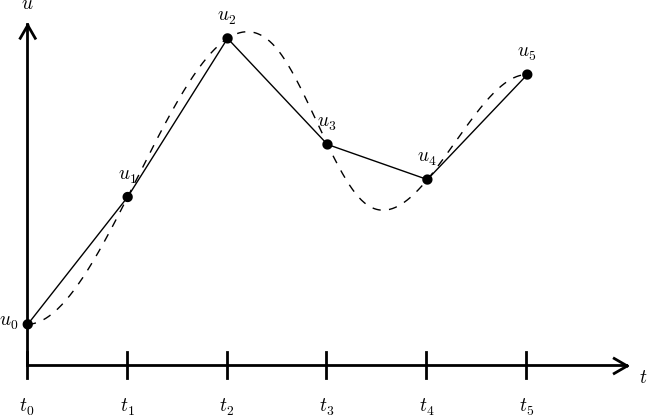
\( u^n \) is a mesh function, defined at the mesh points \( t_n \), \( n=0,\ldots,N_t \) only.

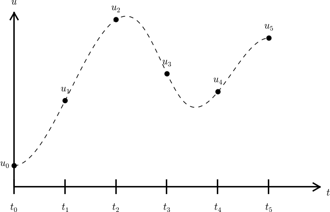
What about a mesh function between the mesh points?

Can extend the mesh function to yield values between mesh points by linear interpolation:

 
$$ \begin{equation} u(t) \approx u^n + \frac{u^{n+1}-u^n}{t_{n+1}-t_n}(t - t_n)\tp \end{equation} $$

Step 2: Fulfilling the equation at discrete time points

• The ODE holds for all \( t\in (0,T] \) (infinite no of points)
• Idea: let the ODE be valid at the mesh points only (finite no of points)

 
$$ \begin{equation} u'(t_n) = -au(t_n),\quad n=1,\ldots,N_t\tp \tag{2} \end{equation} $$

Step 3: Replacing derivatives by finite differences

Now it is time for the finite difference approximations of derivatives:

 
$$ \begin{equation} u'(t_n) \approx \frac{u^{n+1}-u^{n}}{t_{n+1}-t_n}\tp \tag{3} \end{equation} $$

Step 3: Replacing derivatives by finite differences

Inserting the finite difference approximation in

 
$$ u'(t_n) = -au(t_n),$$

 
gives

 
$$ \begin{equation} \frac{u^{n+1}-u^{n}}{t_{n+1}-t_n} = -au^{n},\quad n=0,1,\ldots,N_t-1\tp \tag{4} \end{equation} $$

This is the

• discrete equation
• discrete problem
• finite difference method
• finite difference scheme

Step 4: Formulating a recursive algorithm

• How can we actually compute the \( u^n \) values?
• Fundamental structure:

• given \( u^0=I \)
• compute \( u^1 \) from \( u^0 \)
• compute \( u^2 \) from \( u^1 \)
• compute \( u^3 \) from \( u^2 \) (and so forth)
• In general: we have \( u^n \) and seek \( u^{n+1} \)

Let us apply the scheme

Assume constant time spacing: \( \Delta t = t_{n+1}-t_n=\mbox{const} \)

 
$$ \begin{align*} u_0 &= I,\\ u_1 & = u^0 - a\Delta t u^0 = I(1-a\Delta t),\\ u_2 & = I(1-a\Delta t)^2,\\ u^3 &= I(1-a\Delta t)^3,\\ &\vdots\\ u^{N_t} &= I(1-a\Delta t)^{N_t}\tp \end{align*} $$

Ooops - we can find the numerical solution by hand (in this simple example)! No need for a computer (yet)...

A backward difference

Here is another finite difference approximation to the derivative (backward difference):

 
$$ \begin{equation} u'(t_n) \approx \frac{u^{n}-u^{n-1}}{t_{n}-t_{n-1}}\tp \tag{6} \end{equation} $$

The Backward Euler scheme

Inserting the finite difference approximation in \( u'(t_n)=-au(t_n) \) yields the Backward Euler (BE) scheme:

 
$$ \begin{equation} \frac{u^{n}-u^{n-1}}{t_{n}-t_{n-1}} = -a u^n\tp \tag{7} \end{equation} $$

 
Solve with respect to the unknown \( u^{n+1} \):

 
$$ \begin{equation} u^{n+1} = \frac{1}{1+ a(t_{n+1}-t_n)} u^n\tp \tag{8} \end{equation} $$

A centered difference

Centered differences are better approximations than forward or backward differences.

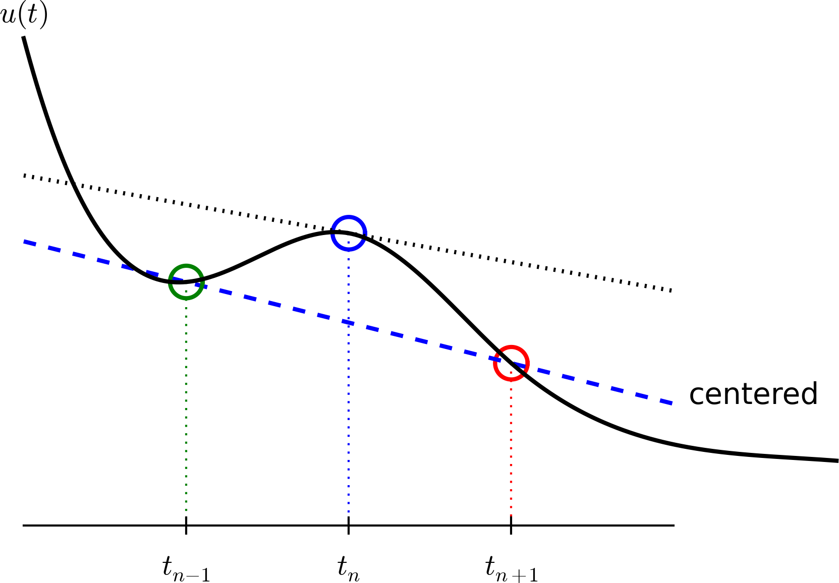
The Crank-Nicolson scheme; part 1

Idea 1: let the ODE hold at \( t_{n+1/2} \)

 
$$ u'(t_{n+1/2} = -au(t_{n+1/2})\tp$$

Idea 2: approximate \( u'(t_{n+1/2} \) by a centered difference

 
$$ \begin{equation} u'(t_{n+\half}) \approx \frac{u^{n+1}-u^n}{t_{n+1}-t_n}\tp \tag{9} \end{equation} $$

Problem: \( u(t_{n+1/2}) \) is not defined, only \( u^n=u(t_n) \) and \( u^{n+1}=u(t_{n+1}) \)

Solution:

 
$$ u(t_{n+1/2}) \approx \half(u^n + u^{n+1}) $$

The Crank-Nicolson scheme; part 2

Result:

 
$$ \begin{equation} \frac{u^{n+1}-u^n}{t_{n+1}-t_n} = -a\half (u^n + u^{n+1})\tp \tag{10} \end{equation} $$

Solve wrt to \( u^{n+1} \):

 
$$ \begin{equation} u^{n+1} = \frac{1-\half a(t_{n+1}-t_n)}{1 + \half a(t_{n+1}-t_n)}u^n\tp \tag{11} \end{equation} $$

 
This is a Crank-Nicolson (CN) scheme or a midpoint or centered scheme.

The unifying \( \theta \)-rule

The Forward Euler, Backward Euler, and Crank-Nicolson schemes can be formulated as one scheme with a varying parameter \( \theta \):

 
$$ \begin{equation} \frac{u^{n+1}-u^{n}}{t_{n+1}-t_n} = -a (\theta u^{n+1} + (1-\theta) u^{n}) \tag{12} \tp \end{equation} $$

• \( \theta =0 \): Forward Euler
• \( \theta =1 \): Backward Euler
• \( \theta =1/2 \): Crank-Nicolson
• We may alternatively choose any \( \theta\in [0,1] \).

\( u^n \) is known, solve for \( u^{n+1} \):

 
$$ \begin{equation} u^{n+1} = \frac{1 - (1-\theta) a(t_{n+1}-t_n)}{1 + \theta a(t_{n+1}-t_n)}\tp \tag{13} \end{equation} $$

Constant time step

Very common assumption (not important, but exclusively used for simplicity hereafter): constant time step \( t_{n+1}-t_n\equiv\Delta t \)

Test the understanding!

Derive Forward Euler, Backward Euler, and Crank-Nicolson schemes for Newton's law of cooling:

 
$$ T' = -k(T-T_s),\quad T(0)=T_0,\ t\in (0,t_{\mbox{end}}]\tp$$

Physical quantities:

• \( T(t) \): temperature of an object at time \( t \)
• \( k \): parameter expressing heat loss to the surroundings
• \( T_s \): temperature of the surroundings
• \( T_0 \): initial temperature

Compact operator notation for finite differences

• Finite difference formulas can be tedious to write and read/understand
• Handy tool: finite difference operator notation
• Advantage: communicates the nature of the difference in a compact way

 
$$ \begin{equation} [D_t^- u = -au]^n \tp \end{equation} $$

Compact operator notation for difference operators

Forward difference:

 
$$ \begin{equation} [D_t^+u]^n = \frac{u^{n+1} - u^{n}}{\Delta t} \approx \frac{d}{dt} u(t_n) \tag{18} \tp \end{equation} $$

 
Centered difference:

 
$$ \begin{equation} [D_tu]^n = \frac{u^{n+\half} - u^{n-\half}}{\Delta t} \approx \frac{d}{dt} u(t_n), \tag{19} \end{equation} $$

Backward difference:

 
$$ \begin{equation} [D_t^-u]^n = \frac{u^{n} - u^{n-1}}{\Delta t} \approx \frac{d}{dt} u(t_n) \tag{20} \end{equation} $$

The Backward Euler scheme with operator notation

 
$$ \begin{equation*} [D_t^-u]^n = -au^n \tp \end{equation*} $$

Common to put the whole equation inside square brackets:

 
$$ \begin{equation} [D_t^- u = -au]^n \tp \end{equation} $$

The Forward Euler scheme with operator notation

 
$$ \begin{equation} [D_t^+ u = -au]^n\tp \end{equation} $$

The Crank-Nicolson scheme with operator notation

Introduce an averaging operator:

 
$$ \begin{equation} [\overline{u}^{t}]^n = \half (u^{n-\half} + u^{n+\half} ) \approx u(t_n) \tag{21} \end{equation} $$

The Crank-Nicolson scheme can then be written as

 
$$ \begin{equation} [D_t u = -a\overline{u}^t]^{n+\half}\tp \tag{22} \end{equation} $$

Test: use the definitions and write out the above formula to see that it really is the Crank-Nicolson scheme!

Implementation

Model:

 
$$ u'(t) = -au(t),\quad t\in (0,T], \quad u(0)=I, $$

Numerical method:

 
$$ u^{n+1} = \frac{1 - (1-\theta) a\Delta t}{1 + \theta a\Delta t}u^n, $$

 
for \( \theta\in [0,1] \). Note

• \( \theta=0 \) gives Forward Euler
• \( \theta=1 \) gives Backward Euler
• \( \theta=1/2 \) gives Crank-Nicolson

Requirements of a program

• Compute the numerical solution \( u^n \), \( n=1,2,\ldots,N_t \)
• Display the numerical and exact solution \( \uex(t)=e^{-at} \)
• Bring evidence to a correct implementation (verification)
• Compare the numerical and the exact solution in a plot
• computes the error \( \uex (t_n) - u^n \)
• computes the convergence rate of the numerical scheme
• reads its input data from the command line

Tools to learn

• Basic Python programming
• Array computing with numpy
• Plotting with matplotlib.pyplot and scitools
• File writing and reading
• Making command-line user interface via argparse.ArgumentParser
• Making graphical user interfaces via Parampool

Why implement in Python?

• Python has a very clean, readable syntax (often known as "executable pseudo-code").
• Python code is very similar to MATLAB code (and MATLAB has a particularly widespread use for scientific computing).
• Python is a full-fledged, very powerful programming language.
• Python is similar to, but much simpler to work with and results in more reliable code than C++.

Why implement in Python?

• Python has a rich set of modules for scientific computing, and its popularity in scientific computing is rapidly growing.
• Python was made for being combined with compiled languages (C, C++, Fortran) to reuse existing numerical software and to reach high computational performance of new implementations.
• Python has extensive support for administrative task needed when doing large-scale computational investigations.
• Python has extensive support for graphics (visualization, user interfaces, web applications).
• FEniCS, a very powerful tool for solving PDEs by the finite element method, is most human-efficient to operate from Python.

Algorithm

• Store \( u^n \), \( n=0,1,\ldots,N_t \) in an array u.
• Algorithm:

1. initialize \( u^0 \)
2. for \( t=t_n \), \( n=1,2,\ldots,N_t \): compute \( u_n \) using the \( \theta \)-rule formula

Translation to Python function

from numpy import *

def solver(I, a, T, dt, theta):
    """Solve u'=-a*u, u(0)=I, for t in (0,T] with steps of dt."""
    Nt = int(T/dt)            # no of time intervals
    T = Nt*dt                 # adjust T to fit time step dt
    u = zeros(Nt+1)           # array of u[n] values
    t = linspace(0, T, Nt+1)  # time mesh

    u[0] = I                  # assign initial condition
    for n in range(0, Nt):    # n=0,1,...,Nt-1
        u[n+1] = (1 - (1-theta)*a*dt)/(1 + theta*dt*a)*u[n]
    return u, t

Note about the for loop: range(0, Nt, s) generates all integers from 0 to Nt in steps of s (default 1), but not including Nt (!).

Sample call:

u, t = solver(I=1, a=2, T=8, dt=0.8, theta=1)

Integer division

Python applies integer division: 1/2 is 0, while 1./2 or 1.0/2 or 1/2. or 1/2.0 or 1.0/2.0 all give 0.5.

A safer solver function (dt = float(dt) - guarantee float):

from numpy import *

def solver(I, a, T, dt, theta):
    """Solve u'=-a*u, u(0)=I, for t in (0,T] with steps of dt."""
    dt = float(dt)            # avoid integer division
    Nt = int(round(T/dt))     # no of time intervals
    T = Nt*dt                 # adjust T to fit time step dt
    u = zeros(Nt+1)           # array of u[n] values
    t = linspace(0, T, Nt+1)  # time mesh

    u[0] = I                  # assign initial condition
    for n in range(0, Nt):    # n=0,1,...,Nt-1
        u[n+1] = (1 - (1-theta)*a*dt)/(1 + theta*dt*a)*u[n]
    return u, t

Doc strings

• First string after the function heading
• Used for documenting the function
• Automatic documentation tools can make fancy manuals for you
• Can be used for automatic testing

def solver(I, a, T, dt, theta):
    """
    Solve

        u'(t) = -a*u(t),

    with initial condition u(0)=I, for t in the time interval
    (0,T]. The time interval is divided into time steps of
    length dt.

    theta=1 corresponds to the Backward Euler scheme, theta=0
    to the Forward Euler scheme, and theta=0.5 to the Crank-
    Nicolson method.
    """
    ...

Formatting of numbers

Can control formatting of reals and integers through the printf format:

print 't=%6.3f u=%g' % (t[i], u[i])

Or the alternative format string syntax:

print 't={t:6.3f} u={u:g}'.format(t=t[i], u=u[i])

Running the program

How to run the program decay_v1.py:

Terminal> python decay_v1.py

Can also run it as "normal" Unix programs: ./decay_v1.py if the first line is

`#!/usr/bin/env python`

Then

Terminal> chmod a+rx decay_v1.py
Terminal> ./decay_v1.py

Verifying the implementation

• Verification = bring evidence that the program works
• Find suitable test problems
• Make function for each test problem
• Later: put the verification tests in a professional testing framework

Simplest method: run a few algorithmic steps by hand

Use a calculator (\( I=0.1 \), \( \theta=0.8 \), \( \Delta t =0.8 \)):

 
$$ A\equiv \frac{1 - (1-\theta) a\Delta t}{1 + \theta a \Delta t} = 0.298245614035$$

 
$$ \begin{align*} u^1 &= AI=0.0298245614035,\\ u^2 &= Au^1= 0.00889504462912,\\ u^3 &=Au^2= 0.00265290804728 \end{align*} $$

See the function verify_three_steps in decay_verf1.py.

Comparison with an exact discrete solution

Define

 
$$ A = \frac{1 - (1-\theta) a\Delta t}{1 + \theta a \Delta t}\tp $$

 
Repeated use of the \( \theta \)-rule:

 
$$ \begin{align*} u^0 &= I,\\ u^1 &= Au^0 = AI,\\ u^n &= A^nu^{n-1} = A^nI \tp \end{align*} $$

Making a test based on an exact discrete solution

The exact discrete solution as

 
$$ \begin{equation} u^n = IA^n \tag{23} \tp \end{equation} $$

Test if

 
$$ \max_n |u^n - \uex(t_n)| < \epsilon\sim 10^{-15}$$

Implementation in decay_verf2.py.

Test the understanding!

Make a program for solving Newton's law of cooling

 
$$ T' = -k(T-T_s),\quad T(0)=T_0,\ t\in (0,t_{\mbox{end}}]\tp$$

 
with the Forward Euler, Backward Euler, and Crank-Nicolson schemes (or a \( \theta \) scheme). Verify the implementation.

Computing the numerical error as a mesh function

Task: compute the numerical error \( e^n = \uex(t_n) - u^n \)

Exact solution: \( \uex(t)=Ie^{-at} \), implemented as

def exact_solution(t, I, a):
    return I*exp(-a*t)

Compute \( e^n \) by

u, t = solver(I, a, T, dt, theta)  # Numerical solution
u_e = exact_solution(t, I, a)
e = u_e - u

Computing the norm of the error

• \( e^n \) is a mesh function
• Usually we want one number for the error
• Use a norm of \( e^n \)

Norms of a function \( f(t) \):

 
$$ \begin{align} ||f||_{L^2} &= \left( \int_0^T f(t)^2 dt\right)^{1/2} \tag{24}\\ ||f||_{L^1} &= \int_0^T |f(t)| dt \tag{25}\\ ||f||_{L^\infty} &= \max_{t\in [0,T]}|f(t)| \tag{26} \end{align} $$

Norms of mesh functions

• Problem: \( f^n =f(t_n) \) is a mesh function and hence not defined for all \( t \). How to integrate \( f^n \)?
• Idea: Apply a numerical integration rule, using only the mesh points of the mesh function.

The Trapezoidal rule:

 
$$ ||f^n|| = \left(\Delta t\left(\half(f^0)^2 + \half(f^{N_t})^2 + \sum_{n=1}^{N_t-1} (f^n)^2\right)\right)^{1/2} $$

Common simplification yields the \( L^2 \) norm of a mesh function:

 
$$ ||f^n||_{\ell^2} = \left(\Delta t\sum_{n=0}^{N_t} (f^n)^2\right)^{1/2} \tp$$

Implementation of the norm of the error

 
$$ E = ||e^n||_{\ell^2} = \sqrt{\Delta t\sum_{n=0}^{N_t} (e^n)^2}$$

Python w/array arithmetics:

e = u_exact(t) - u
E = sqrt(dt*sum(e**2))

Comment on array vs scalar computation

Scalar computing of E = sqrt(dt*sum(e**2)):

m = len(u)     # length of u array (alt: u.size)
u_e = zeros(m)
t = 0
for i in range(m):
    u_e[i] = exact_solution(t, a, I)
    t = t + dt
e = zeros(m)
for i in range(m):
    e[i] = u_e[i] - u[i]
s = 0  # summation variable
for i in range(m):
    s = s + e[i]**2
error = sqrt(dt*s)

Obviously, scalar computing

• takes more code
• is less readable
• runs much slower

Plotting solutions

Basic plotting with Matplotlib is much like MATLAB plotting

from matplotlib.pyplot import *
plot(t, u)
show()

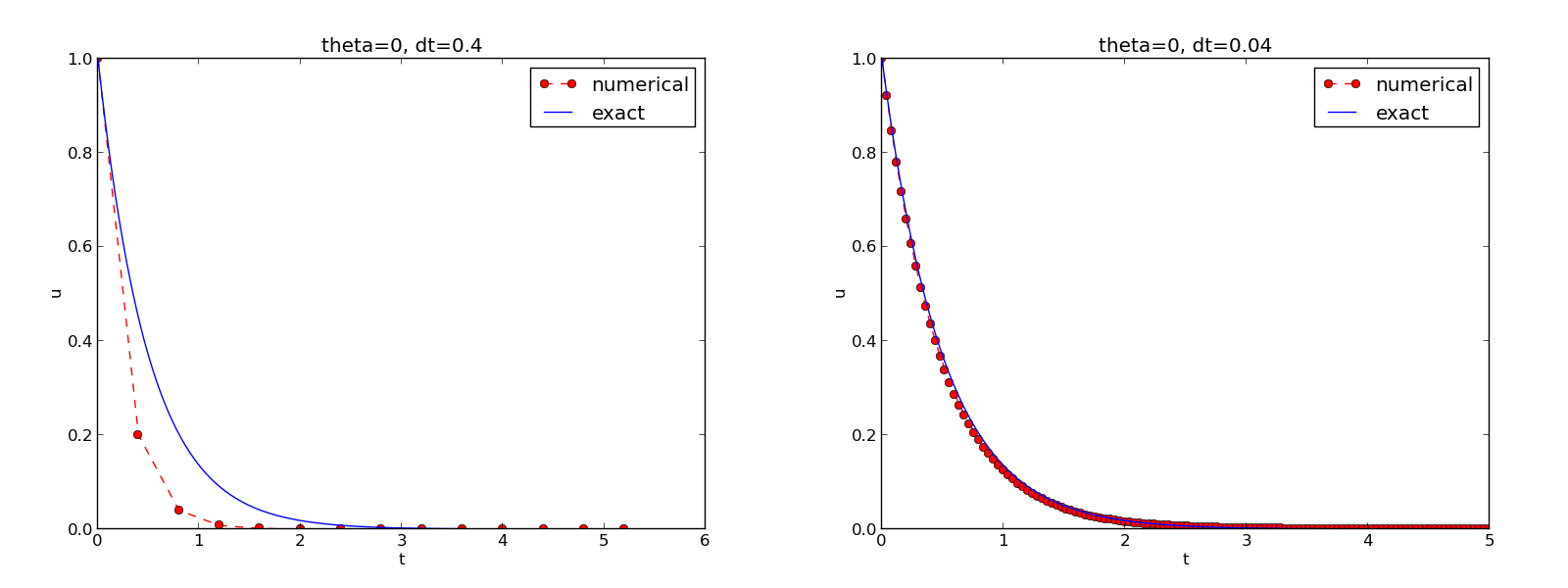
Compare u curve with \( \uex(t) \):

t_e = linspace(0, T, 1001)      # fine mesh
u_e = exact_solution(t_e, I, a)
plot(t_e, u_e, 'b-')            # blue line for u_e
plot(t,   u,   'r--o')          # red dashes w/circles

Decorating a plot

• Use different line types
• Add axis labels
• Add curve legends
• Add plot title
• Save plot to file

from matplotlib.pyplot import *

figure()                          # create new plot
t_e = linspace(0, T, 1001)        # fine mesh for u_e
u_e = exact_solution(t_e, I, a)
plot(t,   u,   'r--o')            # red dashes w/circles
plot(t_e, u_e, 'b-')              # blue line for exact sol.
legend(['numerical', 'exact'])
xlabel('t')
ylabel('u')
title('theta=%g, dt=%g' % (theta, dt))
savefig('%s_%g.png' % (theta, dt))
show()

See complete code in decay_plot_mpl.py.

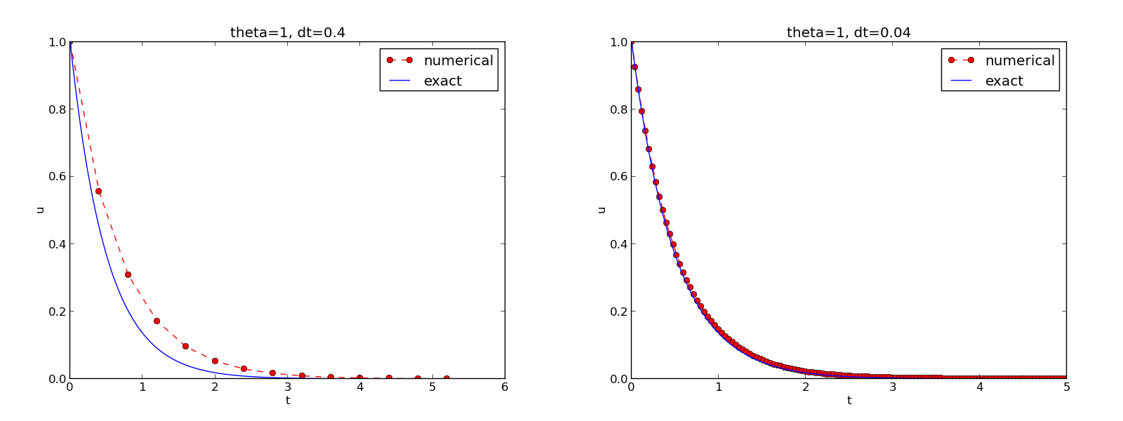
How the plots look like

Plotting with SciTools

SciTools provides a unified plotting interface (Easyviz) to many different plotting packages: Matplotlib, Gnuplot, Grace, VTK, OpenDX, ...

Can use Matplotlib (MATLAB-like) syntax, or a more compact plot function syntax:

from scitools.std import *

plot(t,   u,   'r--o',           # red dashes w/circles
     t_e, u_e, 'b-',             # blue line for exact sol.
     legend=['numerical', 'exact'],
     xlabel='t',
     ylabel='u',
     title='theta=%g, dt=%g' % (theta, dt),
     savefig='%s_%g.png' % (theta2name[theta], dt),
     show=True)

Complete code in decay_plot_st.py.

Change backend (plotting engine, Matplotlib by default):

Terminal> python decay_plot_st.py --SCITOOLS_easyviz_backend gnuplot
Terminal> python decay_plot_st.py --SCITOOLS_easyviz_backend grace

Creating user interfaces

• Never edit the program to change input!
• Set input data on the command line or in a graphical user interface
• How is explained next

Accessing command-line arguments

• All command-line arguments are available in sys.argv
• sys.argv[0] is the program
• sys.argv[1:] holds the command-line arguments
• Method 1: fixed sequence of parameters on the command line
• Method 2: --option value pairs on the command line (with default values)

Terminal> python myprog.py 1.5 2 0.5 0.8 0.4
Terminal> python myprog.py --I 1.5 --a 2 --dt 0.8 0.4

Reading a sequence of command-line arguments

The program decay_plot_mpl.py needs this input:

• \( I \)
• \( a \)
• \( T \)
• an option to turn the plot on or off (makeplot)
• a list of \( \Delta t \) values

Give these on the command line in correct sequence

Terminal> python decay_cml.py 1.5 2 0.5 0.8 0.4

Implementation

import sys

def read_command_line():
    if len(sys.argv) < 6:
        print 'Usage: %s I a T on/off dt1 dt2 dt3 ...' % \ 
              sys.argv[0]; sys.exit(1)  # abort

    I = float(sys.argv[1])
    a = float(sys.argv[2])
    T = float(sys.argv[3])
    makeplot = sys.argv[4] in ('on', 'True')
    dt_values = [float(arg) for arg in sys.argv[5:]]

    return I, a, T, makeplot, dt_values

Note:

• sys.argv[i] is always a string
• Must explicitly convert to (e.g.) float for computations
• List comprehensions make lists: [expression for e in somelist]

Complete program: decay_cml.py.

Working with an argument parser

Set option-value pairs on the command line if the default value is not suitable:

Terminal> python decay_argparse.py --I 1.5 --a 2 --dt 0.8 0.4

Code:

def define_command_line_options():
    import argparse
    parser = argparse.ArgumentParser()
    parser.add_argument('--I', '--initial_condition', type=float,
                        default=1.0, help='initial condition, u(0)',
                        metavar='I')
    parser.add_argument('--a', type=float,
                        default=1.0, help='coefficient in ODE',
                        metavar='a')
    parser.add_argument('--T', '--stop_time', type=float,
                        default=1.0, help='end time of simulation',
                        metavar='T')
    parser.add_argument('--makeplot', action='store_true',
                        help='display plot or not')
    parser.add_argument('--dt', '--time_step_values', type=float,
                        default=[1.0], help='time step values',
                        metavar='dt', nargs='+', dest='dt_values')
    return parser

(metavar is the symbol used in help output)

Reading option-values pairs

argparse.ArgumentParser parses the command-line arguments:

def read_command_line():
    parser = define_command_line_options()
    args = parser.parse_args()
    print 'I={}, a={}, T={}, makeplot={}, dt_values={}'.format(
        args.I, args.a, args.T, args.makeplot, args.dt_values)
    return args.I, args.a, args.T, args.makeplot, args.dt_values

Complete program: decay_argparse.py.

A graphical user interface

Normally very much programming required - and much competence on graphical user interfaces.

Here: use a tool to automatically create it in a few minutes (!)

The Parampool package

• Parampool is a package for handling a large pool of input parameters in simulation programs
• Parampool can automatically create a sophisticated web-based graphical user interface (GUI) to set parameters and view solutions

Making a compute function

• Key concept: a compute function that takes all input data as arguments and returning HTML code for viewing the results (e.g., plots and numbers)
• What we have: decay_plot_mpl.py
• main function carries out simulations and plotting for a series of \( \Delta t \) values
• Goal: steer and view these experiments from a web GUI
• What to do:

• create a compute function
• call parampool functionality

The compute function main_GUI:

def main_GUI(I=1.0, a=.2, T=4.0,
         dt_values=[1.25, 0.75, 0.5, 0.1],
         theta_values=[0, 0.5, 1]):

The hard part of the compute function: the HTML code

• The results are to be displayed in a web page
• Only you know what to display in your problem
• Therefore, you need to specify the HTML code

Suppose explore solves the problem, makes a plot, computes the error and returns appropriate HTML code with the plot. Embed error and plots in a table:

def main_GUI(I=1.0, a=.2, T=4.0,
         dt_values=[1.25, 0.75, 0.5, 0.1],
         theta_values=[0, 0.5, 1]):
    # Build HTML code for web page. Arrange plots in columns
    # corresponding to the theta values, with dt down the rows
    theta2name = {0: 'FE', 1: 'BE', 0.5: 'CN'}
    html_text = '<table>\n'
    for dt in dt_values:
        html_text += '<tr>\n'
        for theta in theta_values:
            E, html = explore(I, a, T, dt, theta, makeplot=True)
            html_text += """
<td>
<center><b>%s, dt=%g, error: %s</b></center><br>
%s
</td>
""" % (theta2name[theta], dt, E, html)
        html_text += '</tr>\n'
    html_text += '</table>\n'
    return html_text

How to embed a PNG plot in HTML code

In explore:

import matplotlib.pyplot as plt
...
# plot
plt.plot(t, u, r-')
plt.xlabel('t')
plt.ylabel('u')
...
from parampool.utils import save_png_to_str
html_text = save_png_to_str(plt, plotwidth=400)

If you know HTML, you can return more sophisticated layout etc.

Generating the user interface

Make a file decay_GUI_generate.py:

from parampool.generator.flask import generate
from decay_GUI import main
generate(main,
         output_controller='decay_GUI_controller.py',
         output_template='decay_GUI_view.py',
         output_model='decay_GUI_model.py')

Running decay_GUI_generate.py results in

1. decay_GUI_model.py defines HTML widgets to be used to set input data in the web interface,
2. templates/decay_GUI_views.py defines the layout of the web page,
3. decay_GUI_controller.py runs the web application.

Good news: we only need to run decay_GUI_controller.py and there is no need to look into any of these files!

Running the web application

Start the GUI

Terminal> python decay_GUI_controller.py

Open a web browser at 127.0.0.1:5000

More advanced use

• The compute function can have arguments of type float, int, string, list, dict, numpy array, filename (file upload)
• Alternative: specify a hierarchy of input parameters with name, default value, data type, widget type, unit (m, kg, s), validity check
• The generated web GUI can have user accounts with login and storage of results in a database

Computing convergence rates

Frequent assumption on the relation between the numerical error \( E \) and some discretization parameter \( \Delta t \):

 
$$ \begin{equation} E = C\Delta t^r, \tag{27} \end{equation} $$

• Unknown: \( C \) and \( r \).
• Goal: estimate \( r \) (and \( C \)) from numerical experiments

Estimating the convergence rate \( r \)

Perform numerical experiments: \( (\Delta t_i, E_i) \), \( i=0,\ldots,m-1 \). Two methods for finding \( r \) (and \( C \)):

1. Take the logarithm of (27), \( \ln E = r\ln \Delta t + \ln C \), and fit a straight line to the data points \( (\Delta t_i, E_i) \), \( i=0,\ldots,m-1 \).
2. Consider two consecutive experiments, \( (\Delta t_i, E_i) \) and \( (\Delta t_{i-1}, E_{i-1}) \). Dividing the equation \( E_{i-1}=C\Delta t_{i-1}^r \) by \( E_{i}=C\Delta t_{i}^r \) and solving for \( r \) yields

 
$$ \begin{equation} r_{i-1} = \frac{\ln (E_{i-1}/E_i)}{\ln (\Delta t_{i-1}/\Delta t_i)} \tag{28} \end{equation} $$

 
for \( i=1,=\ldots,m-1 \).

Method 2 is best.

Implementation

Compute \( r_0, r_1, \ldots, r_{m-2} \):

from math import log

def main():
    I, a, T, makeplot, dt_values = read_command_line()
    r = {}  # estimated convergence rates
    for theta in 0, 0.5, 1:
        E_values = []
        for dt in dt_values:
            E = explore(I, a, T, dt, theta, makeplot=False)
            E_values.append(E)

        # Compute convergence rates
        m = len(dt_values)
        r[theta] = [log(E_values[i-1]/E_values[i])/
                    log(dt_values[i-1]/dt_values[i])
                    for i in range(1, m, 1)]

    for theta in r:
        print '\nPairwise convergence rates for theta=%g:' % theta
        print ' '.join(['%.2f' % r_ for r_ in r[theta]])
    return r

Complete program: decay_convrate.py.

Execution

Terminal> python decay_convrate.py --dt 0.5 0.25 0.1 0.05 0.025 0.01
...
Pairwise convergence rates for theta=0:
1.33 1.15 1.07 1.03 1.02

Pairwise convergence rates for theta=0.5:
2.14 2.07 2.03 2.01 2.01

Pairwise convergence rates for theta=1:
0.98 0.99 0.99 1.00 1.00

Debugging via convergence rates

Potential bug: missing a in the denominator,

u[n+1] = (1 - (1-theta)*a*dt)/(1 + theta*dt)*u[n]

Running decay_convrate.py gives same rates.

Why? The value of \( a \)... (\( a=1 \))

0 and 1 are bad values in tests!

Better:

Terminal> python decay_convrate.py --a 2.1 --I 0.1  \ 
          --dt 0.5 0.25 0.1 0.05 0.025 0.01
...
Pairwise convergence rates for theta=0:
1.49 1.18 1.07 1.04 1.02

Pairwise convergence rates for theta=0.5:
-1.42 -0.22 -0.07 -0.03 -0.01

Pairwise convergence rates for theta=1:
0.21 0.12 0.06 0.03 0.01

Forward Euler works...because \( \theta=0 \) hides the bug.

This bug gives \( r\approx 0 \):

u[n+1] = ((1-theta)*a*dt)/(1 + theta*dt*a)*u[n]

Memory-saving implementation

• Note 1: we store the entire array u, i.e., \( u^n \) for \( n=0,1,\ldots,N_t \)
• Note 2: the formula for \( u^{n+1} \) needs \( u^n \) only, not \( u^{n-1} \), \( u^{n-2} \), ...
• No need to store more than \( u^{n+1} \) and \( u^{n} \)
• Extremely important when solving PDEs
• No practical importance here (much memory available)
• But let's illustrate how to do save memory!
• Idea 1: store \( u^{n+1} \) in u, \( u^n \) in u_1 (float)
• Idea 2: store u in a file, read file later for plotting

Memory-saving solver function

def solver_memsave(I, a, T, dt, theta, filename='sol.dat'):
    """
    Solve u'=-a*u, u(0)=I, for t in (0,T] with steps of dt.
    Minimum use of memory. The solution is stored in a file
    (with name filename) for later plotting.
    """
    dt = float(dt)         # avoid integer division
    Nt = int(round(T/dt))  # no of intervals

    outfile = open(filename, 'w')
    # u: time level n+1, u_1: time level n
    t = 0
    u_1 = I
    outfile.write('%.16E  %.16E\n' % (t, u_1))
    for n in range(1, Nt+1):
        u = (1 - (1-theta)*a*dt)/(1 + theta*dt*a)*u_1
        u_1 = u
        t += dt
        outfile.write('%.16E  %.16E\n' % (t, u))
    outfile.close()
    return u, t

Reading computed data from file

def read_file(filename='sol.dat'):
    infile = open(filename, 'r')
    u = [];  t = []
    for line in infile:
        words = line.split()
        if len(words) != 2:
            print 'Found more than two numbers on a line!', words
            sys.exit(1)  # abort
        t.append(float(words[0]))
        u.append(float(words[1]))
    return np.array(t), np.array(u)

Simpler code with numpy functionality for reading/writing tabular data:

def read_file_numpy(filename='sol.dat'):
    data = np.loadtxt(filename)
    t = data[:,0]
    u = data[:,1]
    return t, u

Similar function np.savetxt, but then we need all \( u^n \) and \( t^n \) values in a two-dimensional array (which we try to prevent now!).

Usage of memory-saving code

def explore(I, a, T, dt, theta=0.5, makeplot=True):
    filename = 'u.dat'
    u, t = solver_memsave(I, a, T, dt, theta, filename)

    t, u = read_file(filename)
    u_e = exact_solution(t, I, a)
    e = u_e - u
    E = np.sqrt(dt*np.sum(e**2))
    if makeplot:
        plt.figure()
        ...

Complete program: decay_memsave.py.

Software engineering

Goal: make more professional numerical software.

Topics:

• How to make modules (reusable libraries)
• Testing frameworks (doctest, nose, unittest)
• Implementation with classes

Making a module

• Previous programs: much repetitive code (esp. solver)
• DRY (Don't Repeat Yourself) principle: no copies of code
• A change needs to be done in one and only one place
• Module = just a file with functions (reused through import)
• Let's make a module by putting these functions in a file:

• solver
• verify_three_steps
• verify_discrete_solution
• explore
• define_command_line_options
• read_command_line
• main (with convergence rates)
• verify_convergence_rate

Module name: decay_mod, filename: decay_mod.py.

Sketch:

from numpy import *
from matplotlib.pyplot import *
import sys

def solver(I, a, T, dt, theta):
    ...

def verify_three_steps():
    ...

def verify_exact_discrete_solution():
    ...

def exact_solution(t, I, a):
    ...

def explore(I, a, T, dt, theta=0.5, makeplot=True):
    ...

def define_command_line_options():
    ...

def read_command_line(use_argparse=True):
    ...

def main():
    ...

That is! It's a module decay_mod in file decay_mod.py.

Usage in some other program:

from decay_mod import solver
u, t = solver(I=1.0, a=3.0, T=3, dt=0.01, theta=0.5)

Test block

At the end of a module it is common to include a test block:

if __name__ == '__main__':
    main()

• If decay_mod is imported, __name__ is decay_mod.
• If decay_mod.py is run, __name__ is __main__.
• Use test block for testing, demo, user interface, ...

Extended test block:

if __name__ == '__main__':
    if 'verify' in sys.argv:
        if verify_three_steps() and verify_discrete_solution():
            pass # ok
        else:
            print 'Bug in the implementation!'
    elif 'verify_rates' in sys.argv:
        sys.argv.remove('verify_rates')
        if not '--dt' in sys.argv:
            print 'Must assign several dt values'
            sys.exit(1)  # abort
        if verify_convergence_rate():
            pass
        else:
            print 'Bug in the implementation!'
    else:
        # Perform simulations
        main()

Prefixing imported functions by the module name

from numpy import *
from matplotlib.pyplot import *

This imports a large number of names (sin, exp, linspace, plot, ...).

Confusion: is a function from`numpy`? Or matplotlib.pyplot?

Alternative (recommended) import:

import numpy
import matplotlib.pyplot

Now we need to prefix functions with module name:

t = numpy.linspace(0, T, Nt+1)
u_e = I*numpy.exp(-a*t)
matplotlib.pyplot.plot(t, u_e)

Common standard:

import numpy as np
import matplotlib.pyplot as plt

t = np.linspace(0, T, Nt+1)
u_e = I*np.exp(-a*t)
plt.plot(t, u_e)

Downside of module prefix notation

A math line like \( e^{-at}\sin(2\pi t) \) gets cluttered with module names,

numpy.exp(-a*t)*numpy.sin(2(numpy.pi*t)
# or
np.exp(-a*t)*np.sin(2*np.pi*t)

Solution (much used in this course): do two imports

import numpy as np
from numpy import exp, sin, pi
...
t = np.linspace(0, T, Nt+1)
u_e = exp(-a*t)*sin(2*pi*t)

Doctests

Doc strings can be equipped with interactive Python sessions for demonstrating usage and automatic testing of functions.

def solver(I, a, T, dt, theta):
    """
    Solve u'=-a*u, u(0)=I, for t in (0,T] with steps of dt.


    >>> u, t = solver(I=0.8, a=1.2, T=4, dt=0.5, theta=0.5)
    >>> for t_n, u_n in zip(t, u):
    ...     print 't=%.1f, u=%.14f' % (t_n, u_n)
    t=0.0, u=0.80000000000000
    t=0.5, u=0.43076923076923
    t=1.0, u=0.23195266272189
    t=1.5, u=0.12489758761948
    t=2.0, u=0.06725254717972
    t=2.5, u=0.03621291001985
    t=3.0, u=0.01949925924146
    t=3.5, u=0.01049960113002
    t=4.0, u=0.00565363137770
    """
    ...

Running doctests

Automatic check that the code reproduces the doctest output:

Terminal> python -m doctest decay_mod_doctest.py

Report in case of failure:

Terminal> python -m doctest decay_mod_doctest.py
********************************************************
File "decay_mod_doctest.py", line 12, in decay_mod_doctest....
Failed example:
    for t_n, u_n in zip(t, u):
        print 't=%.1f, u=%.14f' % (t_n, u_n)
Expected:
    t=0.0, u=0.80000000000000
    t=0.5, u=0.43076923076923
    t=1.0, u=0.23195266272189
    t=1.5, u=0.12489758761948
    t=2.0, u=0.06725254717972
Got:
    t=0.0, u=0.80000000000000
    t=0.5, u=0.43076923076923
    t=1.0, u=0.23195266272189
    t=1.5, u=0.12489758761948
    t=2.0, u=0.06725254718756
********************************************************
1 items had failures:
   1 of   2 in decay_mod_doctest.solver
***Test Failed*** 1 failures.

Complete program: decay_mod_doctest.py.

Unit testing with nose

• Nose is a very user-friendly testing framework
• Based on unit testing
• Identify (small) units of code and test each unit
• Nose automates running all tests
• Good habit: run all tests after (small) edits of a code
• Even better habit: write tests before the code (!)
• Remark: unit testing in scientific computing is not yet well established

Basic use of nose

1. Implement tests in test functions with names starting with test_.
2. Test functions cannot have arguments.
3. Test functions perform assertions on computed results using assert functions from the nose.tools module.
4. Test functions can be in the source code files or be collected in separate files test*.py.

Example on a nose test in the source code

Very simple module mymod (in file mymod.py):

def double(n):
    return 2*n

Write test function in mymod.py:

def double(n):
    return 2*n

import nose.tools as nt

def test_double():
    result = double(4)
    nt.assert_equal(result, 8)

Running

Terminal> nosetests -s mymod

makes the nose tool run all test_*() functions in mymod.py.

Example on a nose test in a separate file

Write the test in a separate file, say test_mymod.py:

import nose.tools as nt
import mymod

def test_double():
    result = mymod.double(4)
    nt.assert_equal(result, 8)

Running

Terminal> nosetests -s

makes the nose tool run all test_*() functions in all files test*.py in the current directory and in all subdirectories (recursevely) with names tests or *_tests.

The habit of writing nose tests

• Put test_*() functions in the module
• When you get many test_*() functions, collect them in tests/test*.py

Purpose of a test function: raise AssertionError if failure

Alternative ways of raising AssertionError if result is not 8:

import nose.tools as nt

def test_double():
    result = ...

    nt.assert_equal(result, 8)    # alternative 1

    assert result == 8            # alternative 2

    if result != 8:               # alternative 3
        raise AssertionError()

Advantages of nose

• Easier to use than other test frameworks
• Tests are written and collected in a compact and structured way
• Large collections of tests, scattered throughout a directory tree can be executed with one command (nosetests -s)
• Nose is a much-adopted standard

Demonstrating nose (ideas)

Aim: test function solver for \( u'=-au \), \( u(0)=I \).

We design three unit tests:

1. A comparison between the computed \( u^n \) values and the exact discrete solution
2. A comparison between the computed \( u^n \) values and precomputed verified reference values
3. A comparison between observed and expected convergence rates

These tests follow very closely the previous verify* functions.

Demonstrating nose (code)

import nose.tools as nt
import decay_mod_unittest as decay_mod
import numpy as np

def exact_discrete_solution(n, I, a, theta, dt):
    """Return exact discrete solution of the theta scheme."""
    dt = float(dt)  # avoid integer division
    factor = (1 - (1-theta)*a*dt)/(1 + theta*dt*a)
    return I*factor**n

def test_exact_discrete_solution():
    """
    Compare result from solver against
    formula for the discrete solution.
    """
    theta = 0.8; a = 2; I = 0.1; dt = 0.8
    N = int(8/dt)  # no of steps
    u, t = decay_mod.solver(I=I, a=a, T=N*dt, dt=dt, theta=theta)
    u_de = np.array([exact_discrete_solution(n, I, a, theta, dt)
                     for n in range(N+1)])
    diff = np.abs(u_de - u).max()
    nt.assert_almost_equal(diff, 0, delta=1E-14)

Floats as test results require careful comparison

• Round-off errors make exact comparison of floats unreliable
• nt.assert_almost_equal: compare two floats to some digits or precision

def test_solver():
    """
    Compare result from solver against
    precomputed arrays for theta=0, 0.5, 1.
    """
    I=0.8; a=1.2; T=4; dt=0.5  # fixed parameters
    precomputed = {
        't': np.array([ 0. ,  0.5,  1. ,  1.5,  2. ,  2.5,
                        3. ,  3.5,  4. ]),
        0.5: np.array(
            [ 0.8       ,  0.43076923,  0.23195266, 0.12489759,
              0.06725255,  0.03621291,  0.01949926, 0.0104996 ,
              0.00565363]),
        0: ...,
        1: ...
        }
    for theta in 0, 0.5, 1:
        u, t = decay_mod.solver(I, a, T, dt, theta=theta)
        diff = np.abs(u - precomputed[theta]).max()
        # Precomputed numbers are known to 8 decimal places
        nt.assert_almost_equal(diff, 0, places=8,
                               msg='theta=%s' % theta)

Test of wrong use

• Find input data that may cause trouble and test such cases
• Here: the formula for \( u^{n+1} \) may involve integer division

Example:

theta = 1; a = 1; I = 1; dt = 2

may lead to integer division:

(1 - (1-theta)*a*dt)  # becomes 1
(1 + theta*dt*a)      # becomes 2
(1 - (1-theta)*a*dt)/(1 + theta*dt*a)  # becomes 0 (!)

Test that solver does not suffer from such integer division:

def test_potential_integer_division():
    """Choose variables that can trigger integer division."""
    theta = 1; a = 1; I = 1; dt = 2
    N = 4
    u, t = decay_mod.solver(I=I, a=a, T=N*dt, dt=dt, theta=theta)
    u_de = np.array([exact_discrete_solution(n, I, a, theta, dt)
                     for n in range(N+1)])
    diff = np.abs(u_de - u).max()
    nt.assert_almost_equal(diff, 0, delta=1E-14)

Test of convergence rates

Convergence rate tests are very common for differential equation solvers.

def test_convergence_rates():
    """Compare empirical convergence rates to exact ones."""
    # Set command-line arguments directly in sys.argv
    import sys
    sys.argv[1:] = '--I 0.8 --a 2.1 --T 5 '\ 
                   '--dt 0.4 0.2 0.1 0.05 0.025'.split()
    r = decay_mod.main()
    for theta in r:
        nt.assert_true(r[theta])  # check for non-empty list

    expected_rates = {0: 1, 1: 1, 0.5: 2}
    for theta in r:
        r_final = r[theta][-1]
        # Compare to 1 decimal place
        nt.assert_almost_equal(expected_rates[theta], r_final,
                               places=1, msg='theta=%s' % theta)

Complete program: test_decay_nose.py.

Classical unit testing with unittest

• unittest is a Python module mimicing the classical JUnit class-based unit testing framework from Java
• This is how unit testing is normally done
• Requires knowledge of object-oriented programming

Basic use of unittest

Write file test_mymod.py:

import unittest
import mymod

class TestMyCode(unittest.TestCase):
    def test_double(self):
        result = mymod.double(4)
        self.assertEqual(result, 8)

if __name__ == '__main__':
    unittest.main()

Demonstration of unittest

import unittest
import decay_mod_unittest as decay
import numpy as np

def exact_discrete_solution(n, I, a, theta, dt):
    factor = (1 - (1-theta)*a*dt)/(1 + theta*dt*a)
    return I*factor**n

class TestDecay(unittest.TestCase):

    def test_exact_discrete_solution(self):
        ...
        diff = np.abs(u_de - u).max()
        self.assertAlmostEqual(diff, 0, delta=1E-14)

    def test_solver(self):
        ...
        for theta in 0, 0.5, 1:
            ...
            self.assertAlmostEqual(diff, 0, places=8,
                                   msg='theta=%s' % theta)

    def test_potential_integer_division():
        ...
        self.assertAlmostEqual(diff, 0, delta=1E-14)

    def test_convergence_rates(self):
        ...
        for theta in r:
            ...
            self.assertAlmostEqual(...)

if __name__ == '__main__':
    unittest.main()

Complete program: test_decay_unittest.py.

Implementing simple problem and solver classes

• So far: programs are built of Python functions
• New focus: alternative implementations using classes
• Class-based implementations are very popular, especially in business/adm applications
• Class-based implementations scales better to large and complex scientific applications

What to learn

Tasks:

• Explain basic use of classes to build a differential equation solver
• Introduce concepts that make such programs easily scale to more complex applications
• Demonstrate the advantage of using classes

Ideas:

• Classes for Problem, Solver, and Visualizer
• Problem: all the physics information about the problem
• Solver: all the numerics information + numerical computations
• Visualizer: plot the solution and other quantities

The problem class

• Model problem: \( u'=-au \), \( u(0)=I \), for \( t\in (0,T] \).
• Class Problem stores the physical parameters \( a \), \( I \), \( T \)
• May also offer other data, e.g., \( \uex(t)=Ie^{-at} \)

Implementation:

from numpy import exp

class Problem:
    def __init__(self, I=1, a=1, T=10):
        self.T, self.I, self.a = I, float(a), T

    def exact_solution(self, t):
        I, a = self.I, self.a     # extract local variables
        return I*exp(-a*t)

Basic usage:

problem = Problem(T=5)
problem.T = 8
problem.dt = 1.5

Improved problem class

More flexible input from the command line:

class Problem:
    def __init__(self, I=1, a=1, T=10):
        self.T, self.I, self.a = I, float(a), T

    def define_command_line_options(self, parser=None):
        if parser is None:
            import argparse
            parser = argparse.ArgumentParser()

        parser.add_argument(
            '--I', '--initial_condition', type=float,
            default=self.I, help='initial condition, u(0)',
            metavar='I')
        parser.add_argument(
            '--a', type=float, default=self.a,
            help='coefficient in ODE', metavar='a')
        parser.add_argument(
            '--T', '--stop_time', type=float, default=self.T,
            help='end time of simulation', metavar='T')
        return parser

    def init_from_command_line(self, args):
        self.I, self.a, self.T = args.I, args.a, args.T

    def exact_solution(self, t):
        I, a = self.I, self.a
        return I*exp(-a*t)

• Can utilize user's ArgumentParser, or make one
• None is used to indicate a non-initialized variable

The solver class

• Store numerical data \( \Delta t \), \( \theta \)
• Compute solution and quantities derived from the solution

Implementation:

class Solver:
    def __init__(self, problem, dt=0.1, theta=0.5):
        self.problem = problem
        self.dt, self.theta = float(dt), theta

    def define_command_line_options(self, parser):
        parser.add_argument(
            '--dt', '--time_step_value', type=float,
            default=0.5, help='time step value', metavar='dt')
        parser.add_argument(
            '--theta', type=float, default=0.5,
            help='time discretization parameter', metavar='dt')
        return parser

    def init_from_command_line(self, args):
        self.dt, self.theta = args.dt, args.theta

    def solve(self):
        from decay_mod import solver
        self.u, self.t = solver(
            self.problem.I, self.problem.a, self.problem.T,
            self.dt, self.theta)

Note: reuse of the numerical algorithm from the decay_mod module (i.e., the class is a wrapper of the procedural implementation).

The visualizer class

class Visualizer:
    def __init__(self, problem, solver):
        self.problem, self.solver = problem, solver

    def plot(self, include_exact=True, plt=None):
        """
        Add solver.u curve to the plotting object plt,
        and include the exact solution if include_exact is True.
        This plot function can be called several times (if
        the solver object has computed new solutions).
        """
        if plt is None:
            import scitools.std  as plt # can use matplotlib as well

        plt.plot(self.solver.t, self.solver.u, '--o')
        plt.hold('on')
        theta2name = {0: 'FE', 1: 'BE', 0.5: 'CN'}
        name = theta2name.get(self.solver.theta, '')
        legends = ['numerical %s' % name]
        if include_exact:
            t_e = linspace(0, self.problem.T, 1001)
            u_e = self.problem.exact_solution(t_e)
            plt.plot(t_e, u_e, 'b-')
            legends.append('exact')
        plt.legend(legends)
        plt.xlabel('t')
        plt.ylabel('u')
        plt.title('theta=%g, dt=%g' %
                  (self.solver.theta, self.solver.dt))
        plt.savefig('%s_%g.png' % (name, self.solver.dt))
        return plt

Remark: The plt object in plot adds a new curve to a plot, which enables comparing different solutions from different runs of Solver.solve

Combing the classes

Let Problem, Solver, and Visualizer play together:

def main():
    problem = Problem()
    solver = Solver(problem)
    viz = Visualizer(problem, solver)

    # Read input from the command line
    parser = problem.define_command_line_options()
    parser = solver. define_command_line_options(parser)
    args = parser.parse_args()
    problem.init_from_command_line(args)
    solver. init_from_command_line(args)

    # Solve and plot
    solver.solve()
    import matplotlib.pyplot as plt
    #import scitools.std as plt
    plt = viz.plot(plt=plt)
    E = solver.error()
    if E is not None:
        print 'Error: %.4E' % E
    plt.show()

Complete program: decay_class.py.

Implementing more advanced problem and solver classes

• The previous Problem and Solver classes soon contain much repetitive code when the number of parameters increases
• Much of such code can be parameterized and be made more compact
• Idea: collect all parameters in a dictionary self.prms, with two associated dictionaries self.types and self.help for holding associated object types and help strings
• Collect common code in class Parameters
• Let Problem, Solver, and maybe Visualizer be subclasses of class Parameters, basically defining self.prms, self.types, self.help

A generic class for parameters

class Parameters:
    def set(self, **parameters):
        for name in parameters:
            self.prms[name] = parameters[name]

    def get(self, name):
        return self.prms[name]

    def define_command_line_options(self, parser=None):
        if parser is None:
            import argparse
            parser = argparse.ArgumentParser()

        for name in self.prms:
            tp = self.types[name] if name in self.types else str
            help = self.help[name] if name in self.help else None
            parser.add_argument(
                '--' + name, default=self.get(name), metavar=name,
                type=tp, help=help)

        return parser

    def init_from_command_line(self, args):
        for name in self.prms:
            self.prms[name] = getattr(args, name)

Slightly more advanced version in class_decay_verf1.py.

The problem class

class Problem(Parameters):
    """
    Physical parameters for the problem u'=-a*u, u(0)=I,
    with t in [0,T].
    """
    def __init__(self):
        self.prms = dict(I=1, a=1, T=10)
        self.types = dict(I=float, a=float, T=float)
        self.help = dict(I='initial condition, u(0)',
                         a='coefficient in ODE',
                         T='end time of simulation')

    def exact_solution(self, t):
        I, a = self.get('I'), self.get('a')
        return I*np.exp(-a*t)

The solver class

class Solver(Parameters):
    def __init__(self, problem):
        self.problem = problem
        self.prms = dict(dt=0.5, theta=0.5)
        self.types = dict(dt=float, theta=float)
        self.help = dict(dt='time step value',
                         theta='time discretization parameter')

    def solve(self):
        from decay_mod import solver
        self.u, self.t = solver(
            self.problem.get('I'),
            self.problem.get('a'),
            self.problem.get('T'),
            self.get('dt'),
            self.get('theta'))

    def error(self):
        try:
            u_e = self.problem.exact_solution(self.t)
            e = u_e - self.u
            E = np.sqrt(self.get('dt')*np.sum(e**2))
        except AttributeError:
            E = None
        return E

The visualizer class

• No parameters needed (for this simple problem), no need to inherit class Parameters
• Same code as previously shown class Visualizer
• Same code as previously shown for combining Problem, Solver, and Visualizer

Performing scientific experiments

Goal: explore the behavior of a numerical method for a differential equation and show how scientific experiments can be set up and reported.

Tasks:

• Write scripts to automate experiments
• Generate scientific reports from scripts

Tools to learn:

• os.system for running other programs
• subprocess for running other programs and extracting the output
• List comprehensions
• Formats for scientific reports: HTML w/MathJax, LaTeX, Sphinx, Doconce

Model problem and numerical solution method

Problem:

 
$$ \begin{equation} u'(t) = -au(t),\quad u(0)=I,\ 0< t \leq T, \tag{29} \end{equation} $$

Solution method (\( \theta \)-rule):

 
$$ u^{n+1} = \frac{1 - (1-\theta) a\Delta t}{1 + \theta a\Delta t}u^n, \quad u^0=I\tp $$

Plan for the experiments

• Plot \( u^n \) against \( \uex = Ie^{-at} \) for various choices of the parameters \( I \), \( a \), \( \Delta t \), and \( \theta \)
• How does the discrete solution compare with the exact solution when \( \Delta t \) is varied and \( \theta=0,0.5,1 \)?
• Use the decay_mod.py module (little modification of the plotting, see experiments/decay_mod.py)
• Make separate program for running (automating) the experiments (script)

1. python decay_mod.py --I 1 --a 2 --makeplot --T 5 --dt 0.5 0.25 0.1 0.05
2. Combine generated figures FE_*.png, BE_*.png, and CN_*.png to new figures with multiple plots
3. Run script as python decay_exper0.py 0.5 0.25 0.1 0.05 (\( \Delta t \) values on the command line)

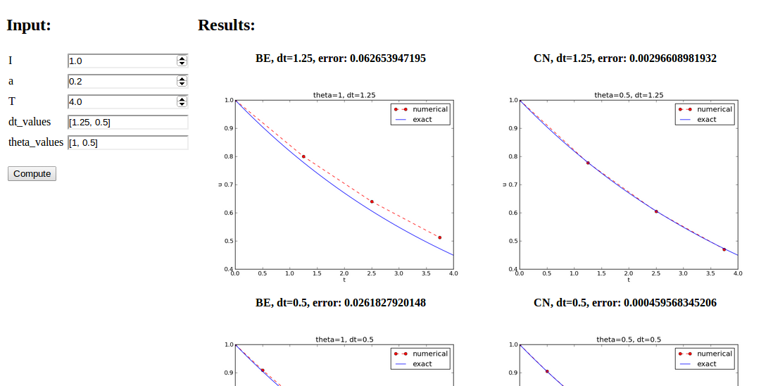
Typical plot summarizing the results

Script code

Typical script (small administering program) for running the experiments:

import os, sys

def run_experiments(I=1, a=2, T=5):
    # The command line must contain dt values
    if len(sys.argv) > 1:
        dt_values = [float(arg) for arg in sys.argv[1:]]
    else:
        print 'Usage: %s dt1 dt2 dt3 ...' %  sys.argv[0]
        sys.exit(1)  # abort

    # Run module file as a stand-alone application
    cmd = 'python decay_mod.py --I %g --a %g --makeplot --T %g' % \
          (I, a, T)
    dt_values_str = ' '.join([str(v) for v in dt_values])
    cmd += ' --dt %s' % dt_values_str
    print cmd
    failure = os.system(cmd)
    if failure:
        print 'Command failed:', cmd; sys.exit(1)

    # Combine images into rows with 2 plots in each row
    image_commands = []
    for method in 'BE', 'CN', 'FE':
        pdf_files = ' '.join(['%s_%g.pdf' % (method, dt)
                              for dt in dt_values])
        png_files = ' '.join(['%s_%g.png' % (method, dt)
                              for dt in dt_values])
        image_commands.append(
            'montage -background white -geometry 100%' +
            ' -tile 2x %s %s.png' % (png_files, method))
        image_commands.append(
            'convert -trim %s.png %s.png' % (method, method))
        image_commands.append(
            'convert %s.png -transparent white %s.png' %
            (method, method))
        image_commands.append(
            'pdftk %s output tmp.pdf' % pdf_files)
        num_rows = int(round(len(dt_values)/2.0))
        image_commands.append(
            'pdfnup --nup 2x%d tmp.pdf' % num_rows)
        image_commands.append(
            'pdfcrop tmp-nup.pdf %s.pdf' % method)

    for cmd in image_commands:
        print cmd
        failure = os.system(cmd)
        if failure:
            print 'Command failed:', cmd; sys.exit(1)

    # Remove the files generated above and by decay_mod.py
    from glob import glob
    filenames = glob('*_*.png') + glob('*_*.pdf') + \
                glob('*_*.eps') + glob('tmp*.pdf')
    for filename in filenames:
        os.remove(filename)

if __name__ == '__main__':
    run_experiments()

Complete program: experiments/decay_exper0.py.

Comments to the code

Many useful constructs in the previous script:

• [float(arg) for arg in sys.argv[1:]] builds a list of real numbers from all the command-line arguments
• failure = os.system(cmd) runs an operating system command (e.g., another program)
• sys.exit(1) aborts the program
• ['%s_%s.png' % (method, dt) for dt in dt_values] builds a list of filenames from a list of numbers (dt_values)
• All montage commands for creating composite figures are stored in a list and thereafter executed in a loop
• glob.glob('*_*.png') returns a list of the names of all files in the current folder where the filename matches the Unix wildcard notation *_*.png (meaning "any text, underscore, any text, and then `.png`")
• os.remove(filename) removes the file with name filename

Interpreting output from other programs

In decay_exper0.py we run a program (os.system) and want to grab the output, e.g.,

Terminal> python decay_plot_mpl.py
0.0   0.40:    2.105E-01
0.0   0.04:    1.449E-02
0.5   0.40:    3.362E-02
0.5   0.04:    1.887E-04
1.0   0.40:    1.030E-01
1.0   0.04:    1.382E-02

Tasks:

• read the output from the decay_mod.py program
• interpret this output and store the \( E \) values in arrays for each \( \theta \) value
• plot \( E \) versus \( \Delta t \), for each \( \theta \), in a log-log plot

Code for grabbing output from another program

Use the subprocess module to grab output:

    from subprocess import Popen, PIPE, STDOUT
    p = Popen(cmd, shell=True, stdout=PIPE, stderr=STDOUT)
    output, dummy = p.communicate()
    failure = p.returncode
    if failure:
        print 'Command failed:', cmd; sys.exit(1)

Code for interpreting the grabbed output

• Run through the output string, line by line
• If the current line prints \( \theta \), \( \Delta t \), and \( E \), split the line into these three pieces and store the data
• Store data in a dictionary errors with keys dt and the three \( \theta \) values

errors = {'dt': dt_values, 1: [], 0: [], 0.5: []}
for line in output.splitlines():
    words = line.split()
    if words[0] in ('0.0', '0.5', '1.0'):  # line with E?
        # typical line: 0.0   1.25:    7.463E+00
        theta = float(words[0])
        E = float(words[2])
        errors[theta].append(E)

Next: plot \( E \) versus \( \Delta t \) for \( \theta=0,0.5,1 \)

Complete program: experiments/decay_exper1.py. Fine recipe for

• how to run other programs
• how to extract and interpret output from other programs
• how to automate many manual steps in creating simulations and figures

Making a report

• Scientific investigations are best documented in a report!
• A sample report
• How can we write such a report?
• First problem: what format should I write in?
• Plain HTML, generated by decay_exper1_html.py
• HTML with MathJax, generated by decay_exper1_mathjax.py
• LaTeX PDF, based on LaTeX source
• Sphinx HTML, based on reStructuredText
• Markdown, MediaWiki, ...
• Doconce can generate LaTeX, HTML w/MathJax, Sphinx, Markdown, MediaWiki, ... (Doconce source for the examples above, and Python program for generating the Doconce source)
• Examples on different report formats

Publishing a complete project

• Make folder (directory) tree
• Keep track of all files via a version control system (Mercurial, Git, ...)
• Publish as private or public repository
• Utilize Bitbucket, Googlecode, GitHub, or similar
• See the intro to such tools

Analysis of finite difference equations

Model:

 
$$ \begin{equation} u'(t) = -au(t),\quad u(0)=I, \end{equation} $$

Method:

 
$$ \begin{equation} u^{n+1} = \frac{1 - (1-\theta) a\Delta t}{1 + \theta a\Delta t}u^n \tag{30} \end{equation} $$

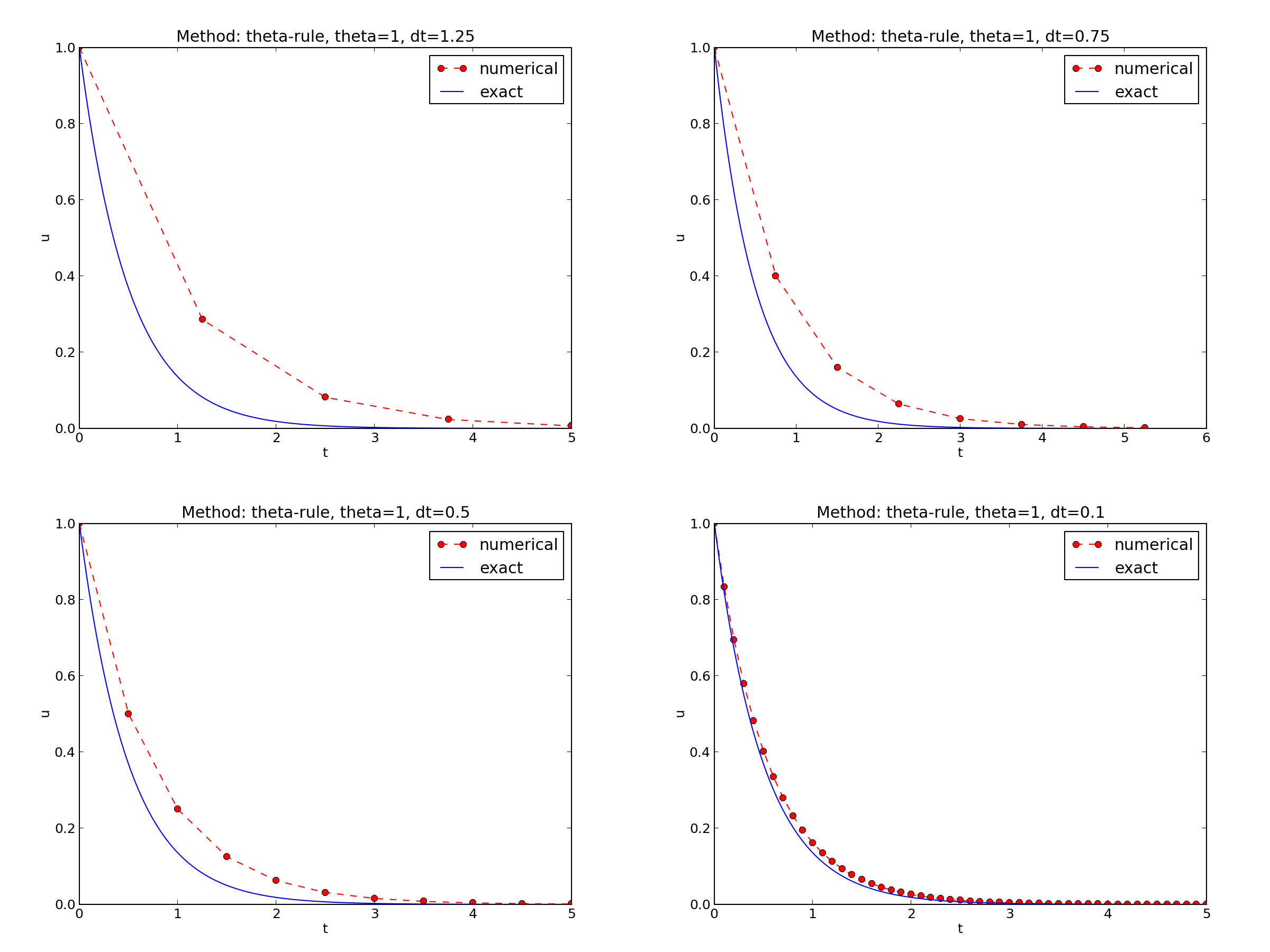
Encouraging numerical solutions

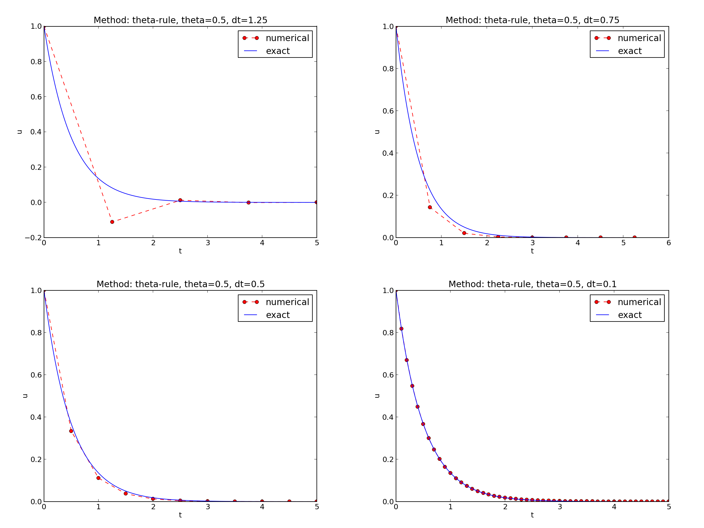
\( I=1 \), \( a=2 \), \( \theta =1,0.5, 0 \), \( \Delta t=1.25, 0.75, 0.5, 0.1 \).

Discouraging numerical solutions; Crank-Nicolson

Discouraging numerical solutions; Forward Euler

Summary of observations

The characteristics of the displayed curves can be summarized as follows:

• The Backward Euler scheme always gives a monotone solution, lying above the exact curve.
• The Crank-Nicolson scheme gives the most accurate results, but for \( \Delta t=1.25 \) the solution oscillates.
• The Forward Euler scheme gives a growing, oscillating solution for \( \Delta t=1.25 \); a decaying, oscillating solution for \( \Delta t=0.75 \); a strange solution \( u^n=0 \) for \( n\geq 1 \) when \( \Delta t=0.5 \); and a solution seemingly as accurate as the one by the Backward Euler scheme for \( \Delta t = 0.1 \), but the curve lies below the exact solution.

Problem setting

Experimental investigation of oscillatory solutions

The solution is oscillatory if

 
$$ u^{n} > u^{n-1},$$

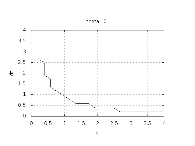
Seems that \( a\Delta t < 1 \) for FE and 2 for CN.

Exact numerical solution

Starting with \( u^0=I \), the simple recursion (30) can be applied repeatedly \( n \) times, with the result that

 
$$ \begin{equation} u^{n} = IA^n,\quad A = \frac{1 - (1-\theta) a\Delta t}{1 + \theta a\Delta t}\tp \tag{31} \end{equation} $$

Such an exact discrete solution is unusual, but very handy for analysis.

Stability

Since \( u^n\sim A^n \),

• \( A<0 \) gives a factor \( (-1)^n \) and oscillatory solutions
• \( |A|>1 \) gives growing solutions
• Recall: the exact solution is monotone and decaying
• If these qualitative properties are not met, we say that the numerical solution is unstable

Computation of stability in this problem

\( A<0 \) if

 
$$ \frac{1 - (1-\theta) a\Delta t}{1 + \theta a\Delta t} < 0 $$

 
To avoid oscillatory solutions we must have \( A> 0 \) and

 
$$ \begin{equation} \Delta t < \frac{1}{(1-\theta)a}\tp \end{equation} $$

• Always fulfilled for Backward Euler
• \( \Delta t \leq 1/a \) for Forward Euler
• \( \Delta t \leq 2/a \) for Crank-Nicolson

Computation of stability in this problem

\( |A|\leq 1 \) means \( -1\leq A\leq 1 \)

 
$$ \begin{equation} -1\leq\frac{1 - (1-\theta) a\Delta t}{1 + \theta a\Delta t} \leq 1\tp \tag{32} \end{equation} $$

 
\( -1 \) is the critical limit:

 
$$ \begin{align*} \Delta t &\leq \frac{2}{(1-2\theta)a},\quad \theta < \half\\ \Delta t &\geq \frac{2}{(1-2\theta)a},\quad \theta > {\half} \end{align*} $$

• Always fulfilled for Backward Euler and Crank-Nicolson
• \( \Delta t \leq 2/a \) for Forward Euler

Explanation of problems with Forward Euler

• \( a\Delta t= 2\cdot 1.25=2.5 \) and \( A=-1.5 \): oscillations and growth
• \( a\Delta t = 2\cdot 0.75=1.5 \) and \( A=-0.5 \): oscillations and decay
• \( \Delta t=0.5 \) and \( A=0 \): \( u^n=0 \) for \( n>0 \)
• Smaller \( Delta t \): qualitatively correct solution

Explanation of problems with Crank-Nicolson

• \( \Delta t=1.25 \) and \( A=-0.25 \): oscillatory solution
• Never any growing solution

Summary of stability

1. Forward Euler is conditionally stable

• \( \Delta t < 2/a \) for avoiding growth
• \( \Delta t\leq 1/a \) for avoiding oscillations
2. The Crank-Nicolson is unconditionally stable wrt growth and conditionally stable wrt oscillations

• \( \Delta t < 2/a \) for avoiding oscillations
3. Backward Euler is unconditionally stable

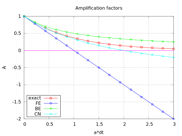
Comparing amplification factors

\( u^{n+1} \) is an amplification \( A \) of \( u^n \):

 
$$ u^{n+1} = Au^n,\quad A = \frac{1 - (1-\theta) a\Delta t}{1 + \theta a\Delta t} $$

The exact solution is also an amplification:

 
$$ u(t_{n+1}) = \Aex u(t_n), \quad \Aex = e^{-a\Delta t}$$

A possible measure of accuracy: \( \Aex - A \)

Plot of amplification factors

Series expansion of amplification factors

To investigate \( \Aex - A \) mathematically, we can Taylor expand the expression, using \( p=a\Delta t \) as variable.

>>> from sympy import *
>>> # Create p as a mathematical symbol with name 'p'
>>> p = Symbol('p')
>>> # Create a mathematical expression with p
>>> A_e = exp(-p)
>>>
>>> # Find the first 6 terms of the Taylor series of A_e
>>> A_e.series(p, 0, 6)
1 + (1/2)*p**2 - p - 1/6*p**3 - 1/120*p**5 + (1/24)*p**4 + O(p**6)

>>> theta = Symbol('theta')
>>> A = (1-(1-theta)*p)/(1+theta*p)
>>> FE = A_e.series(p, 0, 4) - A.subs(theta, 0).series(p, 0, 4)
>>> BE = A_e.series(p, 0, 4) - A.subs(theta, 1).series(p, 0, 4)
>>> half = Rational(1,2)  # exact fraction 1/2
>>> CN = A_e.series(p, 0, 4) - A.subs(theta, half).series(p, 0, 4)
>>> FE
(1/2)*p**2 - 1/6*p**3 + O(p**4)
>>> BE
-1/2*p**2 + (5/6)*p**3 + O(p**4)
>>> CN
(1/12)*p**3 + O(p**4)

Error in amplification factors

Focus: the error measure \( A-\Aex \) as function of \( \Delta t \) (recall that \( p=a\Delta t \)):

 
$$ \begin{equation} A-\Aex = \left\lbrace\begin{array}{ll} \Oof{\Delta t^2}, & \hbox{Forward and Backward Euler},\\ \Oof{\Delta t^3}, & \hbox{Crank-Nicolson} \end{array}\right. \end{equation} $$

The fraction of numerical and exact amplification factors

Focus: the error measure \( 1-A/\Aex \) as function of \( p=a\Delta t \):

>>> FE = 1 - (A.subs(theta, 0)/A_e).series(p, 0, 4)
>>> BE = 1 - (A.subs(theta, 1)/A_e).series(p, 0, 4)
>>> CN = 1 - (A.subs(theta, half)/A_e).series(p, 0, 4)
>>> FE
(1/2)*p**2 + (1/3)*p**3 + O(p**4)
>>> BE
-1/2*p**2 + (1/3)*p**3 + O(p**4)
>>> CN
(1/12)*p**3 + O(p**4)

Same leading-order terms as for the error measure \( A-\Aex \).

The true/global error at a point

• The error in \( A \) reflects the local error when going from one time step to the next
• What is the global (true) error at \( t_n \)? \( e^n = \uex(t_n) - u^n = Ie^{-at_n} - IA^n \)
• Taylor series expansions of \( e^n \) simplify the expression

Computing the global error at a point

>>> n = Symbol('n')
>>> u_e = exp(-p*n)   # I=1
>>> u_n = A**n        # I=1
>>> FE = u_e.series(p, 0, 4) - u_n.subs(theta, 0).series(p, 0, 4)
>>> BE = u_e.series(p, 0, 4) - u_n.subs(theta, 1).series(p, 0, 4)
>>> CN = u_e.series(p, 0, 4) - u_n.subs(theta, half).series(p, 0, 4)
>>> FE
(1/2)*n*p**2 - 1/2*n**2*p**3 + (1/3)*n*p**3 + O(p**4)
>>> BE
(1/2)*n**2*p**3 - 1/2*n*p**2 + (1/3)*n*p**3 + O(p**4)
>>> CN
(1/12)*n*p**3 + O(p**4)

Substitute \( n \) by \( t/\Delta t \):

• Forward and Backward Euler: leading order term \( \half ta^2\Delta t \)
• Crank-Nicolson: leading order term \( \frac{1}{12}ta^3\Delta t^2 \)

Convergence

The numerical scheme is convergent if the global error \( e^n\rightarrow 0 \) as \( \Delta t\rightarrow 0 \). If the error has a leading order term \( \Delta t^r \), the convergence rate is of order \( r \).

Integrated errors

Focus: norm of the numerical error

 
$$ ||e^n||_{\ell^2} = \sqrt{\Delta t\sum_{n=0}^{N_t} ({\uex}(t_n) - u^n)^2} \tp $$

Forward and Backward Euler:

 
$$ ||e^n||_{\ell^2} = \frac{1}{4}\sqrt{\frac{T^3}{3}} a^2\Delta t\tp$$

Crank-Nicolson:

 
$$ ||e^n||_{\ell^2} = \frac{1}{12}\sqrt{\frac{T^3}{3}}a^3\Delta t^2\tp$$

Truncation error

• How good is the discrete equation?
• Possible answer: see how well \( \uex \) fits the discrete equation

 
$$ \lbrack D_t u = -au\rbrack^n,$$

 
i.e.,

 
$$ \frac{u^{n+1}-u^n}{\Delta t} = -au^n\tp$$

 
Insert \( \uex \) (which does not in general fulfill this equation):

 
$$ \begin{equation} \frac{\uex(t_{n+1})-\uex(t_n)}{\Delta t} + a\uex(t_n) = R^n \neq 0 \tp \tag{33} \end{equation} $$

Computation of the truncation error

• The residual \( R^n \) is the truncation error.
• How does \( R^n \) vary with \( \Delta t \)?

Tool: Taylor expand \( \uex \) around the point where the ODE is sampled (here \( t_n \))

 
$$ \uex(t_{n+1}) = \uex(t_n) + \uex'(t_n)\Delta t + \half\uex''(t_n) \Delta t^2 + \cdots $$

 
Inserting this Taylor series in (33) gives

 
$$ R^n = \uex'(t_n) + \half\uex''(t_n)\Delta t + \ldots + a\uex(t_n)\tp$$

 
Now, \( \uex \) solves the ODE \( \uex'=-a\uex \), and then

 
$$ R^n \approx \half\uex''(t_n)\Delta t \tp $$

 
This is a mathematical expression for the truncation error.

The truncation error for other schemes

Backward Euler:

 
$$ R^n \approx -\half\uex''(t_n)\Delta t, $$

Crank-Nicolson:

 
$$ R^{n+\half} \approx \frac{1}{24}\uex'''(t_{n+\half})\Delta t^2\tp$$

Consistency, stability, and convergence

• Truncation error measures the residual in the difference equations. The scheme is consistent if the truncation error goes to 0 as \( \Delta t\rightarrow 0 \). Importance: the difference equations approaches the differential equation as \( \Delta t\rightarrow 0 \).
• Stability means that the numerical solution exhibits the same qualitative properties as the exact solution. Here: monotone, decaying function.
• Convergence implies that the true (global) error \( e^n =\uex(t_n)-u^n\rightarrow 0 \) as \( \Delta t\rightarrow 0 \). This is really what we want!

The Lax equivalence theorem for linear differential equations: consistency + stability is equivalent with convergence.

(Consistency and stability is in most problems much easier to establish than convergence.)

Model extensions

Extension to a variable coefficient; Forward and Backward Euler

 
$$ \begin{equation} u'(t) = -a(t)u(t),\quad t\in (0,T],\quad u(0)=I \tp \tag{34} \end{equation} $$

The Forward Euler scheme:

 
$$ \begin{equation} \frac{u^{n+1} - u^n}{\Delta t} = -a(t_n)u^n \tp \end{equation} $$

The Backward Euler scheme:

 
$$ \begin{equation} \frac{u^{n} - u^{n-1}}{\Delta t} = -a(t_n)u^n \tp \end{equation} $$

Extension to a variable coefficient; Crank-Nicolson

Eevaluting \( a(t_{n+\half}) \) and using an average for \( u \):

 
$$ \begin{equation} \frac{u^{n+1} - u^{n}}{\Delta t} = -a(t_{n+\half})\half(u^n + u^{n+1}) \tp \end{equation} $$

Using an average for \( a \) and \( u \):

 
$$ \begin{equation} \frac{u^{n+1} - u^{n}}{\Delta t} = -\half(a(t_n)u^n + a(t_{n+1})u^{n+1}) \tp \end{equation} $$

Extension to a variable coefficient; \( \theta \)-rule

The \( \theta \)-rule unifies the three mentioned schemes,

 
$$ \begin{equation} \frac{u^{n+1} - u^{n}}{\Delta t} = -a((1-\theta)t_n + \theta t_{n+1})((1-\theta) u^n + \theta u^{n+1}) \tp \end{equation} $$

 
or,

 
$$ \begin{equation} \frac{u^{n+1} - u^{n}}{\Delta t} = -(1-\theta) a(t_n)u^n - \theta a(t_{n+1})u^{n+1} \tp \end{equation} $$

Extension to a variable coefficient; operator notation

 
$$ \begin{align*} \lbrack D^+_t u &= -au\rbrack^n,\\ \lbrack D^-_t u &= -au\rbrack^n,\\ \lbrack D_t u &= -a\overline{u}^t\rbrack^{n+\half},\\ \lbrack D_t u &= -\overline{au}^t\rbrack^{n+\half},\\ \tp \end{align*} $$

Extension to a source term

 
$$ \begin{equation} u'(t) = -a(t)u(t) + b(t),\quad t\in (0,T],\quad u(0)=I \tp \tag{35} \end{equation} $$

 
$$ \begin{align*} \lbrack D^+_t u &= -au + b\rbrack^n,\\ \lbrack D^-_t u &= -au + b\rbrack^n,\\ \lbrack D_t u &= -a\overline{u}^t + b\rbrack^{n+\half},\\ \lbrack D_t u &= \overline{-au+b}^t\rbrack^{n+\half} \tp \end{align*} $$

Implementation of the generalized model problem

 
$$ \begin{equation} u^{n+1} = ((1 - \Delta t(1-\theta)a^n)u^n + \Delta t(\theta b^{n+1} + (1-\theta)b^n))(1 + \Delta t\theta a^{n+1})^{-1} \tp \end{equation} $$

Implementation where \( a(t) \) and \( b(t) \) are given as Python functions (see file decay_vc.py):

def solver(I, a, b, T, dt, theta):
    """
    Solve u'=-a(t)*u + b(t), u(0)=I,
    for t in (0,T] with steps of dt.
    a and b are Python functions of t.
    """
    dt = float(dt)            # avoid integer division
    Nt = int(round(T/dt))     # no of time intervals
    T = Nt*dt                 # adjust T to fit time step dt
    u = zeros(Nt+1)           # array of u[n] values
    t = linspace(0, T, Nt+1)  # time mesh

    u[0] = I                  # assign initial condition
    for n in range(0, Nt):    # n=0,1,...,Nt-1
        u[n+1] = ((1 - dt*(1-theta)*a(t[n]))*u[n] + \ 
                  dt*(theta*b(t[n+1]) + (1-theta)*b(t[n])))/\ 
                  (1 + dt*theta*a(t[n+1]))
    return u, t

Implementations of variable coefficients; functions

Plain functions:

def a(t):
    return a_0 if t < tp else k*a_0

def b(t):
    return 1

Implementations of variable coefficients; classes

Better implementation: class with the parameters a0, tp, and k as attributes and a special method __call__ for evaluating \( a(t) \):

class A:
    def __init__(self, a0=1, k=2):
        self.a0, self.k = a0, k

    def __call__(self, t):
        return self.a0 if t < self.tp else self.k*self.a0

a = A(a0=2, k=1)  # a behaves as a function a(t)

Implementations of variable coefficients; lambda function

Quick writing: a one-liner lambda function

a = lambda t: a_0 if t < tp else k*a_0

In general,

f = lambda arg1, arg2, ...: expressin

is equivalent to

def f(arg1, arg2, ...):
    return expression

One can use lambda functions directly in calls:

u, t = solver(1, lambda t: 1, lambda t: 1, T, dt, theta)

for a problem \( u'=-u+1 \), \( u(0)=1 \).

A lambda function can appear anywhere where a variable can appear.

Verification via trivial solutions

• Start debugging of a new code with trying a problem where \( u=\hbox{const} \neq 0 \).
• Choose \( u=C \) (a constant). Choose any \( a(t) \) and set \( b=a(t)C \) and \( I=C \).
• "All" numerical methods will reproduce \( u=_{\hbox{const}} \) exactly (machine precision).
• Often \( u=C \) eases debugging.
• In this example: any error in the formula for \( u^{n+1} \) make \( u\neq C \)!

Verification via trivial solutions; nose test

import nose.tools as nt

def test_constant_solution():
    """
    Test problem where u=u_const is the exact solution, to be
    reproduced (to machine precision) by any relevant method.
    """
    def exact_solution(t):
        return u_const

    def a(t):
        return 2.5*(1+t**3)  # can be arbitrary

    def b(t):
        return a(t)*u_const

    u_const = 2.15
    theta = 0.4; I = u_const; dt = 4
    Nt = 4  # enough with a few steps
    u, t = solver(I=I, a=a, b=b, T=Nt*dt, dt=dt, theta=theta)
    print u
    u_e = exact_solution(t)
    difference = abs(u_e - u).max()  # max deviation
    nt.assert_almost_equal(difference, 0, places=14)

Verification via manufactured solutions

• Choose any formula for \( u(t) \).
• Fit \( I \), \( a(t) \), and \( b(t) \) in \( u'=-au+b \), \( u(0)=I \), to make the chosen formula a solution of the ODE problem.
• Then we can always have an analytical solution (!).
• Ideal for verification: testing convergence rates.
• Called the method of manufactured solutions (MMS)
• Special case: \( u \) linear in \( t \), because all sound numerical methods will reproduce a linear \( u \) exactly (machine precision).
• \( u(t) = ct + d \). \( u(0)=0 \) means \( d=I \).
• ODE implies \( c = -a(t)u + b(t) \).
• Choose \( a(t) \) and \( c \), and set \( b(t) = c + a(t)(ct + I) \).
• Any error in the formula for \( u^{n+1} \) makes \( u\neq ct+I \)!

Linear manufactured solution

\( u^n = ct_n+I \) fulfills the discrete equations!

First,

 
$$ \begin{align} \lbrack D_t^+ t\rbrack^n &= \frac{t_{n+1}-t_n}{\Delta t}=1, \tag{36}\\ \lbrack D_t^- t\rbrack^n &= \frac{t_{n}-t_{n-1}}{\Delta t}=1, \tag{37}\\ \lbrack D_t t\rbrack^n &= \frac{t_{n+\half}-t_{n-\half}}{\Delta t}=\frac{(n+\half)\Delta t - (n-\half)\Delta t}{\Delta t}=1\tag{38} \tp \end{align} $$

Forward Euler:

 
$$ [D^+ u = -au + b]^n, $$

\( a^n=a(t_n) \), \( b^n=c + a(t_n)(ct_n + I) \), and \( u^n=ct_n + I \) results in

 
$$ c = -a(t_n)(ct_n+I) + c + a(t_n)(ct_n + I) = c $$

Nose test for linear manufactured solution

def test_linear_solution():
    """
    Test problem where u=c*t+I is the exact solution, to be
    reproduced (to machine precision) by any relevant method.
    """
    def exact_solution(t):
        return c*t + I

    def a(t):
        return t**0.5  # can be arbitrary

    def b(t):
        return c + a(t)*exact_solution(t)

    theta = 0.4; I = 0.1; dt = 0.1; c = -0.5
    T = 4
    Nt = int(T/dt)  # no of steps
    u, t = solver(I=I, a=a, b=b, T=Nt*dt, dt=dt, theta=theta)
    u_e = exact_solution(t)
    difference = abs(u_e - u).max()  # max deviation
    print difference
    # No of decimal places for comparison depend on size of c
    nt.assert_almost_equal(difference, 0, places=14)

Extension to systems of ODEs

Sample system:

 
$$ \begin{align} u' &= a u + bv,\\ v' &= cu + dv, \end{align} $$

The Forward Euler method:

 
$$ \begin{align} u^{n+1} &= u^n + \Delta t (a u^n + b v^n),\\ v^{n+1} &= u^n + \Delta t (cu^n + dv^n) \tp \end{align} $$

The Backward Euler method gives a system of algebraic equations

The Backward Euler scheme:

 
$$ \begin{align} u^{n+1} &= u^n + \Delta t (a u^{n+1} + b v^{n+1}),\\ v^{n+1} &= v^n + \Delta t (c u^{n+1} + d v^{n+1})\tp \end{align} $$

 
which is a \( 2\times 2 \) linear system:

 
$$ \begin{align} (1 - \Delta t a)u^{n+1} + bv^{n+1} &= u^n ,\\ c u^{n+1} + (1 - \Delta t d) v^{n+1} &= v^n , \end{align} $$

Crank-Nicolson also gives a \( 2\times 2 \) linear system.

General first-order ODEs

Generic form

The standard form for ODEs:

 
$$ \begin{equation} u' = f(u,t),\quad u(0)=I, \tag{39} \end{equation} $$

\( u \) and \( f \): scalar or vector.

Vectors in case of ODE systems:

 
$$ u(t) = (u^{(0)}(t),u^{(1)}(t),\ldots,u^{(m-1)}(t)) \tp $$

 
$$ \begin{align*} f(u, t) = ( & f^{(0)}(u^{(0)},\ldots,u^{(m-1)}),\\ & f^{(1)}(u^{(0)},\ldots,u^{(m-1)}),\\ & \vdots\\ & f^{(m-1)}(u^{(0)}(t),\ldots,u^{(m-1)}(t))) \tp \end{align*} $$

The \( \theta \)-rule

 
$$ \begin{equation} \frac{u^{n+1}-u^n}{\Delta t} = \theta f(u^{n+1},t_{n+1}) + (1-\theta)f(u^n, t_n)\tp \tag{40} \end{equation} $$

 
Bringing the unknown \( u^{n+1} \) to the left-hand side and the known terms on the right-hand side gives

 
$$ \begin{equation} u^{n+1} - \Delta t \theta f(u^{n+1},t_{n+1}) = u^n + \Delta t(1-\theta)f(u^n, t_n)\tp \end{equation} $$

 
This is a nonlinear equation in \( u^{n+1} \) (unless \( f \) is linear in \( u \))!

Implicit 2-step backward scheme

 
$$ u'(t_{n+1}) \approx \frac{3u^{n+1} - 4u^{n} + u^{n-1}}{2\Delta t},$$

Scheme:

 
$$ u^{n+1} = \frac{4}{3}u^n - \frac{1}{3}u^{n-1} + \frac{2}{3}\Delta t f(u^{n+1}, t_{n+1}) \tp \tag{41} $$

 
Nonlinear equation for \( u^{n+1} \).

The Leapfrog scheme

Idea:

 
$$ \begin{equation} u'(t_n)\approx \frac{u^{n+1}-u^{n-1}}{2\Delta t} = [D_{2t} u]^n, \end{equation} $$

Scheme:

 
$$ [D_{2t} u = f(u,t)]^n,$$

 
or written out,

 
$$ \begin{equation} u^{n+1} = u^{n-1} + \Delta t f(u^n, t_n) \tp \tag{42} \end{equation} $$

• Some other scheme must be used as starter (\( u^1 \)).
• Explicit scheme - a nonlinear \( f \) (in \( u \)) is trivial to handle.
• Downside: Leapfrog is always unstable after some time.

The filtered Leapfrog scheme

After computing \( u^{n+1} \), stabilize Leapfrog by

 
$$ \begin{equation} u^n\ \leftarrow\ u^n + \gamma (u^{n-1} - 2u^n + u^{n+1}) \tag{43} \tp \end{equation} $$

2nd-order Runge-Kutta scheme

Forward-Euler + approximate Crank-Nicolson:

 
$$ \begin{align} u^* &= u^n + \Delta t f(u^n, t_n), \tag{44}\\ u^{n+1} &= u^n + \Delta t \half \left( f(u^n, t_n) + f(u^*, t_{n+1}) \right), \tag{45} \end{align} $$

4th-order Runge-Kutta scheme

• The most famous and widely used ODE method
• 4 evaluations of \( f \) per time step
• Its derivation is a very good illustration of numerical thinking!

2nd-order Adams-Bashforth scheme

 
$$ \begin{equation} u^{n+1} = u^n + \half\Delta t\left( 3f(u^n, t_n) - f(u^{n-1}, t_{n-1}) \right) \tp \tag{46} \end{equation} $$

3rd-order Adams-Bashforth scheme

 
$$ \begin{equation} u^{n+1} = u^n + \frac{1}{12}\left( 23f(u^n, t_n) - 16 f(u^{n-1},t_{n-1}) + 5f(u^{n-2}, t_{n-2})\right) \tp \tag{47} \end{equation} $$

The Odespy software

Odespy features simple Python implementations of the most fundamental schemes as well as Python interfaces to several famous packages for solving ODEs: ODEPACK, Vode, rkc.f, rkf45.f, Radau5, as well as the ODE solvers in SciPy, SymPy, and odelab.

Typical usage:

# Define right-hand side of ODE
def f(u, t):
    return -a*u

import odespy
import numpy as np

# Set parameters and time mesh
I = 1; a = 2; T = 6; dt = 1.0
Nt = int(round(T/dt))
t_mesh = np.linspace(0, T, Nt+1)

# Use a 4th-order Runge-Kutta method
solver = odespy.RK4(f)
solver.set_initial_condition(I)
u, t = solver.solve(t_mesh)

Example: Runge-Kutta methods

solvers = [odespy.RK2(f),
           odespy.RK3(f),
           odespy.RK4(f),
           odespy.BackwardEuler(f, nonlinear_solver='Newton')]

for solver in solvers:
    solver.set_initial_condition(I)
    u, t = solver.solve(t)

# + lots of plot code...

Plots from the experiments

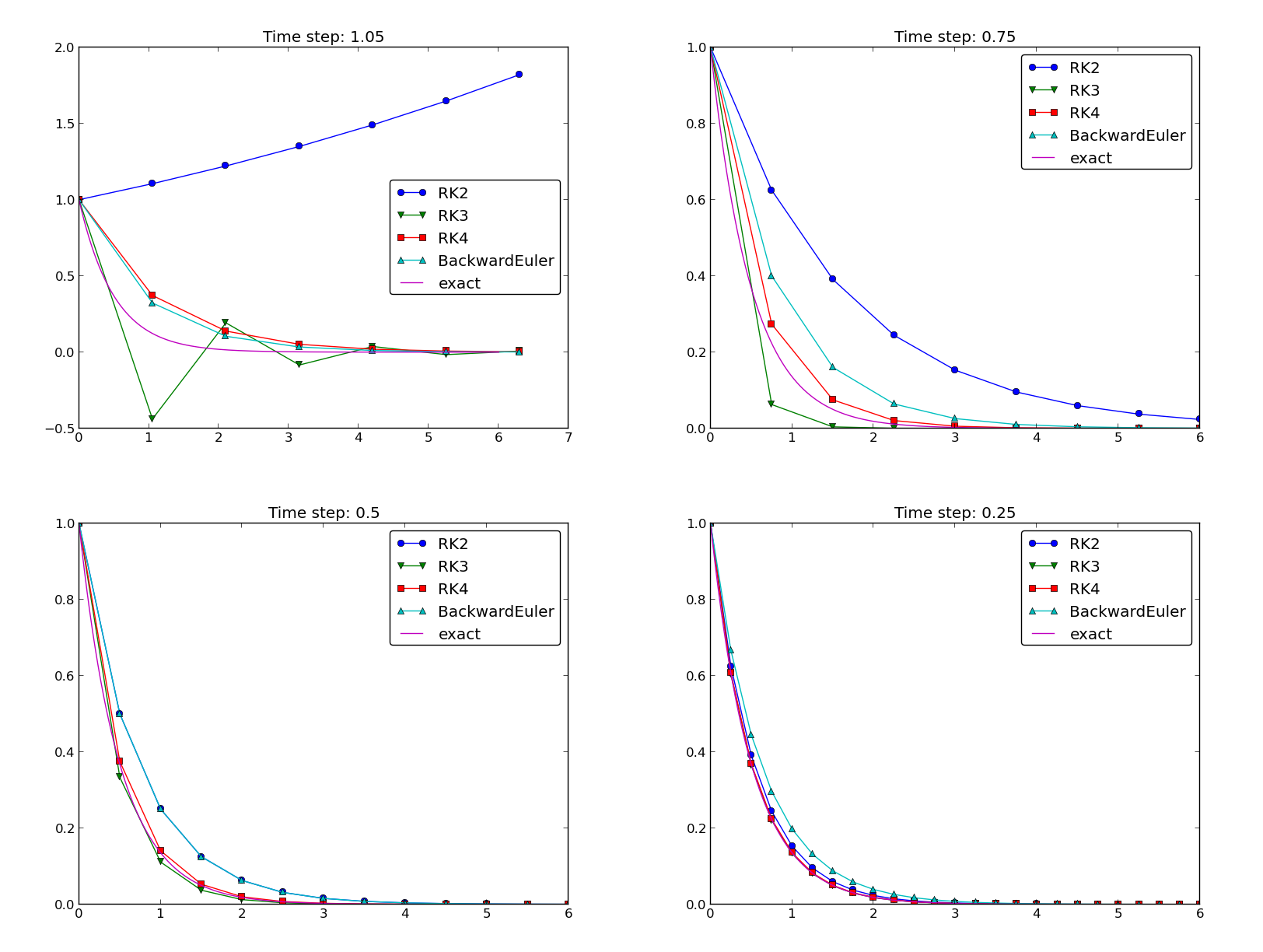
The 4-th order Runge-Kutta method (RK4) is the method of choice!

Example: Adaptive Runge-Kutta methods

• Adaptive methods find "optimal" locations of the mesh points to ensure that the error is less than a given tolerance.
• Downside: approximate error estimation, not always optimal location of points.
• "Industry standard ODE solver": Dormand-Prince 4/5-th order Runge-Kutta (MATLAB's famous ode45).