

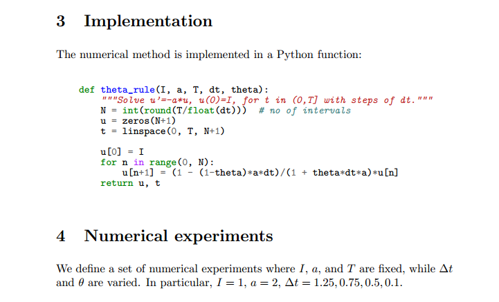
$$ \begin{equation} u'(t) = -au(t),\quad u(0)=I,\quad t\in (0,T], \tag{43} \end{equation} $$ numerically discretized by the \( \theta \)-rule:
$$ u^{n+1} = \frac{1 - (1-\theta) a\Delta t}{1 + \theta a\Delta t}u^n, \quad u^0=I\tp $$ Our aim is to plot \( u^0,u^1,\ldots,u^N \) together with the exact solution \( \uex = Ie^{-at} \) for various choices of the parameters in this numerical problem: \( I \), \( a \), \( \Delta t \), and \( \theta \). We are especially interested in how the discrete solution compares with the exact solution when the \( \Delta t \) parameter is varied and \( \theta \) takes on the three values corresponding to the Forward Euler, Backward Euler, and Crank-Nicolson schemes (\( \theta=0,1,0.5 \), respectively).
A verified implementation for computing the numerical
solution \( u^n \) and plotting it together
with the exact solution \( \uex \) is found in the file
decay_mod.py.
This program admits command-line arguments to specify a series of
\( \Delta t \) values and will run a loop over these values and
\( \theta=0,0.5,1 \). We make a slight edit of how the plots are
designed: the numerical solution is specified with line type 'r--o'
(dashed red lines with dots at the mesh points), and the show()
command is removed to avoid a lot of plot windows popping up on
the computer screen (but hardcopies of the plot are still stored
in files via savefig). The slightly
modified program has the name
experiments/decay_mod.py.
All files associated with the scientific investigation are collected
in a subdirectory experiments.
Running the experiments is easy since the decay_mod.py program
already has the loops over \( \theta \) and \( \Delta t \) implemented.
An experiment with \( I=1 \), \( a=2 \), \( T=5 \), and \( dt=0.5, 0.25, 0.1, 0.05 \)
is run by
Terminal> python decay_mod.py --I 1 --a 2 --makeplot \
          --T 5 --dt 0.5 0.25 0.1 0.05
The decay_mod.py program generates a lot of image files, e.g.,
FE_*.png, BE_*.png, and CN_*.png.
We want to combine all the FE_*.png files in a table
fashion in one file, with two images in each row,
starting with the largest \( \Delta t \) in the upper
left corner and decreasing the value as we go to the right and down.
This can be done using the montage program. The often occurring white areas around the plots can
be cropped away by the convert -trim command.
The remaining white can be made transparent for HTML pages with a
non-white background by the command convert -transparent white.
Also plot files in the PDF format with names FE_*.pdf, BE_*.pdf,
and CN_*.pdf are generated and these should be combined using other
tools: pdftk to combine individual plots into one file with one plot
per page, and pdfnup to combine the pages into a table with multiple
plots per page. The resulting image often has some extra surrounding
white space that can be removed by the pdfcrop program.
The code snippets below contain all details about the
usage of montage, convert, pdftk, pdfnup, and pdfcrop.
Running manual commands is boring, and errors may easily sneak in. Both for automating manual work and documenting the operating system commands we actually issued in the experiment, we should write a script (little program). An alternative is to write the commands into an IPython notebook and use the notebook as the script. A plain script as a standard Python program in a separate text file will be used here.
The script takes a list of \( \Delta t \) values on the command line as input and makes three combined images, one for each \( \theta \) value, displaying the quality of the numerical solution as \( \Delta t \) varies. For example,
Terminal> python decay_exper0.py 0.5 0.25 0.1 0.05
results in images FE.png, CN.png, BE.png,
FE.pdf, CN.pdf, and BE.pdf,
each with four plots corresponding to the four \( \Delta t \) values.
Each plot compares the numerical solution with the exact one.
The latter image is shown in Figure 10.
Figure 10: Illustration of the Backward Euler method for four time step values.

Ideally, the script should be scalable in the sense that it works for any number of \( \Delta t \) values, which is the case for this particular implementation:
import os, sys

def run_experiments(I=1, a=2, T=5):
    # The command line must contain dt values
    if len(sys.argv) > 1:
        dt_values = [float(arg) for arg in sys.argv[1:]]
    else:
        print 'Usage: %s dt1 dt2 dt3 ...' %  sys.argv[0]
        sys.exit(1)  # abort

    # Run module file as a stand-alone application
    cmd = 'python decay_mod.py --I %g --a %g --makeplot --T %g' % \
          (I, a, T)
    dt_values_str = ' '.join([str(v) for v in dt_values])
    cmd += ' --dt %s' % dt_values_str
    print cmd
    failure = os.system(cmd)
    if failure:
        print 'Command failed:', cmd; sys.exit(1)

    # Combine images into rows with 2 plots in each row
    image_commands = []
    for method in 'BE', 'CN', 'FE':
        pdf_files = ' '.join(['%s_%g.pdf' % (method, dt)
                              for dt in dt_values])
        png_files = ' '.join(['%s_%g.png' % (method, dt)
                              for dt in dt_values])
        image_commands.append(
            'montage -background white -geometry 100%' +
            ' -tile 2x %s %s.png' % (png_files, method))
        image_commands.append(
            'convert -trim %s.png %s.png' % (method, method))
        image_commands.append(
            'convert %s.png -transparent white %s.png' %
            (method, method))
        image_commands.append(
            'pdftk %s output tmp.pdf' % pdf_files)
        num_rows = int(round(len(dt_values)/2.0))
        image_commands.append(
            'pdfnup --nup 2x%d tmp.pdf' % num_rows)
        image_commands.append(
            'pdfcrop tmp-nup.pdf %s.pdf' % method)

    for cmd in image_commands:
        print cmd
        failure = os.system(cmd)
        if failure:
            print 'Command failed:', cmd; sys.exit(1)

    # Remove the files generated above and by decay_mod.py
    from glob import glob
    filenames = glob('*_*.png') + glob('*_*.pdf') + \
                glob('*_*.eps') + glob('tmp*.pdf')
    for filename in filenames:
        os.remove(filename)

if __name__ == '__main__':
    run_experiments()
This file is available as experiments/decay_exper0.py.
We may comment upon many useful constructs in this script:
[float(arg) for arg in sys.argv[1:]] builds a list of real numbers
from all the command-line arguments.failure = os.system(cmd) runs an operating system command, e.g.,
another program. The execution is successful only if failure is zero.sys.exit(1).
Any argument different from 0 signifies to the computer's operating system
that our program stopped with a failure.['%s_%s.png' % (method, dt) for dt in dt_values] builds a list of
filenames from a list of numbers (dt_values).montage, convert, pdftk, pdfnup, and pdfcrop
commands for creating
composite figures are stored in a
list and later executed in a loop.glob('*_*.png') returns a list of the names of all files in the
current directory where the filename matches the Unix wildcard notation
*_*.png (meaning any text, underscore, any text, and then .png).os.remove(filename) removes the file with name filename.
Programs that run other programs, like decay_exper0.py does, will often
need to interpret output from those programs. Let us demonstrate how
this is done in Python by extracting the relations between \( \theta \),
\( \Delta t \), and the error \( E \) as written to the terminal window
by the decay_mod.py program, when being executed by
decay_exper0.py. We will
decay_mod.py programos.system(cmd) call does not allow us to read the
output from running cmd. Instead we need to invoke a bit more
involved procedure:
from subprocess import Popen, PIPE, STDOUT
p = Popen(cmd, shell=True, stdout=PIPE, stderr=STDOUT)
output, dummy = p.communicate()
failure = p.returncode
if failure:
    print 'Command failed:', cmd; sys.exit(1)
The command stored in cmd is run and all text that is written to
the standard output and the standard error is available in the
string output. Or in other words, the text in output is what appeared in the
terminal window while running cmd.
Our next task is to run through the output string, line by line,
and if the current line prints \( \theta \), \( \Delta t \), and \( E \),
we split the line into these three pieces and store the data.
The chosen storage structure is a dictionary errors with keys dt
to hold the \( \Delta t \) values in a list, and three \( \theta \) keys to hold
the corresponding \( E \) values in a list. The relevant code lines are
errors = {'dt': dt_values, 1: [], 0: [], 0.5: []}
for line in output.splitlines():
    words = line.split()
    if words[0] in ('0.0', '0.5', '1.0'):  # line with E?
        # typical line: 0.0   1.25:    7.463E+00
        theta = float(words[0])
        E = float(words[2])
        errors[theta].append(E)
Note that we do not bother to store the \( \Delta t \) values as we
read them from output, because we already have these values in
the dt_values list.
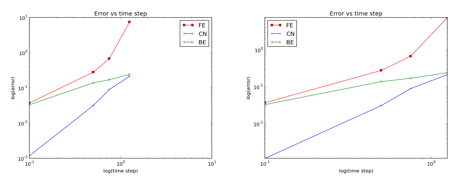
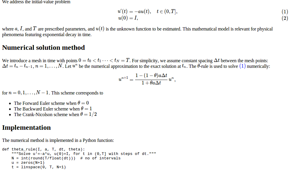
We are now ready to plot \( E \) versus \( \Delta t \) for \( \theta=0,0.5,1 \):
import matplotlib.pyplot as plt
plt.loglog(errors['dt'], errors[0], 'ro-')
plt.hold('on')
plt.loglog(errors['dt'], errors[0.5], 'b+-')
plt.loglog(errors['dt'], errors[1], 'gx-')
plt.legend(['FE', 'CN', 'BE'], loc='upper left')
plt.xlabel('log(time step)')
plt.ylabel('log(error)')
plt.title('Error vs time step')
plt.savefig('error.png')
plt.savefig('error.pdf')
Plots occasionally need some manual adjustments. Here, the axis of the log-log plot look nicer if we adapt them strictly to the data, see Figure 11. To this end, we need to compute \( \min E \) and \( \max E \), and later specify the extent of the axes:
# Find min/max for the axis
E_min = 1E+20; E_max = -E_min
for theta in 0, 0.5, 1:
    E_min = min(E_min, min(errors[theta]))
    E_max = max(E_max, max(errors[theta]))

plt.loglog(errors['dt'], errors[0], 'ro-')
...
plt.axis([min(dt_values), max(dt_values), E_min, E_max])
...
Figure 11: Default plot (left) and manually adjusted axes (right).
The complete program, incorporating the code snippets above, is found
in experiments/decay_exper1.py.
This example can hopefully act as template for numerous
other occasions
where one needs to run experiments, extract data from the output
of programs, make plots, and combine several plots in a figure file.
The decay_exper1.py program
is organized as a module, and other files can then easily extend
the functionality, as illustrated in the next section.
The results of running computer experiments are best documented in a little report containing the problem to be solved, key code segments, and the plots from a series of experiments. At least the part of the report containing the plots should be automatically generated by the script that performs the set of experiments, because in that script we know exactly which input data that were used to generate a specific plot, thereby ensuring that each figure is connected to the right data. Take a look at an example at http://tinyurl.com/k3sdbuv/writing_reports//sphinx-cloud/ to see what we have in mind.
Scientific reports can be written in a variety of formats. Here we
begin with the HTML format
which allows efficient viewing of all the experiments in any web
browser. The program
decay_exper1_html.py calls
decay_exper1.py to perform the experiments and then runs
statements for creating an HTML file with a summary, a
section on the mathematical problem, a section on the numerical
method, a section on the solver function implementing the
method, and a section with subsections containing figures that show
the results of experiments where \( \Delta t \) is varied for
\( \theta=0,0.5,1 \). The mentioned
Python file contains all the details for writing
this HTML report.
You can view the report on http://tinyurl.com/k3sdbuv/writing_reports//_static/report_html.html.
Scientific reports usually need mathematical formulas and hence
mathematical typesetting. In plain HTML, as used in the
decay_exper1_html.py file, we have to use just the keyboard
characters to write mathematics. However, there is an extension to
HTML, called MathJax, which allows
formulas and equations to be typeset with LaTeX syntax and nicely
rendered in web browsers, see Figure
12. A relatively small subset of
LaTeX environments is supported, but the syntax for formulas is quite
rich. Inline formulas are look like \( u'=-au \) while equations are
surrounded by $$ signs. Inside such signs, one can use \[ u'=-au
\] for unnumbered equations, or \begin{equation} and
\end{equation} surrounding u'=-au for numbered equations, or
\begin{align} and \end{align} for multiple aligned equations. You
need to be familiar with mathematical typesetting in LaTeX.
The file decay_exper1_mathjax.py contains all the details for turning the previous plain HTML report into web pages with nicely typeset mathematics. The corresponding HTML code be studied to see all details of the mathematical typesetting.
The de facto language for mathematical typesetting and scientific
report writing is LaTeX. A
number of very sophisticated packages have been added to the language
over a period of three decades, allowing very fine-tuned layout and
typesetting. For output in the PDF format, see Figure
13 for an example, LaTeX is the
definite choice when it comes to quality. The LaTeX language used to
write the reports has typically a lot of commands involving
backslashes and braces. For output on
the web, using HTML (and not the PDF directly in the browser window),
LaTeX struggles with delivering high quality typesetting. Other tools,
especially Sphinx, give better results and can also produce
nice-looking PDFs. The file decay_exper1_latex.py shows how to
generate the LaTeX source from a program.
Figure 13: Report in PDF format generated from LaTeX source.
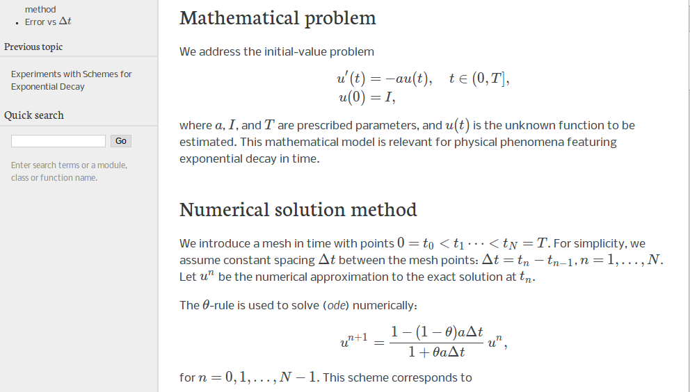
Sphinx is a typesetting language with
similarities to HTML and LaTeX, but with much less tagging. It has
recently become very popular for software documentation and
mathematical reports. Sphinx can utilize LaTeX for mathematical
formulas and equations (via MathJax or PNG images). Unfortunately, the
subset of LaTeX mathematics supported is less than in full MathJax (in
particular, numbering of multiple equations in an align type
environment is not supported). The Sphinx syntax is an extension of
the reStructuredText language. An attractive feature of Sphinx is its
rich support for fancy layout of web pages. In particular,
Sphinx can easily be combined with various layout themes that give a
certain look and feel to the web site and that offers table of
contents, navigation, and search facilities, see Figure
14.
Figure 14: Report in HTML format generated from Sphinx source.
A recently popular format for easy writing of web pages is Markdown. Text is written very much like one would do in email, using spacing and special characters to naturally format the code instead of heavily tagging the text as in LaTeX and HTML. With the tool Pandoc one can go from Markdown to a variety of formats. HTML is a common output format, but LaTeX, epub, XML, OpenOffice, MediaWiki, and MS Word are some other possibilities.
A range of wiki formats are popular for creating notes on the web, especially documents which allow groups of people to edit and add content. Apart from MediaWiki (the wiki format used for Wikipedia), wiki formats have no support for mathematical typesetting and also limited tools for displaying computer code in nice ways. Wiki formats are therefore less suitable for scientific reports compared to the other formats mentioned here.
Since it is difficult to choose the right tool or format for writing
a scientific report, it is advantageous to write the content in a
format that easily translates to LaTeX, HTML, Sphinx, Markdown,
and various wikis. Doconce is such
a tool. It is similar to Pandoc, but offers some special convenient
features for writing about mathematics and programming.
The tagging is modest,
somewhere between LaTeX and Markdown.
The program decay_exper_do.py demonstrates how to generate (and write)
Doconce code for a report.
The HTML, LaTeX (PDF), Sphinx, and Doconce formats for the scientific report whose content is outlined above, are exemplified with source codes and results at the web pages associated with this teaching material: http://tinyurl.com/k3sdbuv/writing_reports/.
A report documenting scientific investigations should be accompanied by all the software and data used for the investigations so that others have a possibility to redo the work and assess the qualify of the results. This possibility is important for reproducible research and hence reaching reliable scientific conclusions.
One way of documenting a complete project is to make a directory tree with all relevant files. Preferably, the tree is published at some project hosting site like Bitbucket, GitHub, or Googlecode so that others can download it as a tarfile, zipfile, or clone the files directly using a version control system like Mercurial or Git. For the investigations outlined in the section Making a report, we can create a directory tree with files
setup.py
./src:
   decay_mod.py
./doc:
   ./src:
      decay_exper1_mathjax.py
      make_report.sh
      run.sh
   ./pub:
      report.html
The src directory holds source code (modules) to be reused in other projects,
the setup.py builds and installs such software,
the doc directory contains the documentation, with src for the
source of the documentation and pub for ready-made, published documentation.
The run.sh file is a simple Bash script listing the python command
we used to run decay_exper1_mathjax.py to generate the experiments and
the report.html file.