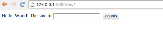
Figure 1: The input page.
Web frameworks
The MVC pattern
A very simple application
Application of the MVC pattern
Making a Flask application
Programming the Flask application
Equipping the input page with output results
Splitting the app into model, view, and controller files
Troubleshooting
Making a Django application
Setting up a Django project
Setting up a Django application
Programming the Django application
Equipping the input page with output results
Handling multiple input variables in Flask
Programming the Flask application
Implementing error checking in the template
Using style sheets
Using LaTeX mathematics
Rearranging the elements in the HTML template
Bootstrap HTML style
Custom validation
Avoiding plot files
Plotting with the Bokeh library
Autogenerating the code
User login and storage of computed results
Uploading of files
Handling multiple input variables in Django
Programming the Django application
Custom validation
Customizing widgets
Resources
Exercises
Exercise 1: Add two numbers
Exercise 2: Upload data file and visualize curves
Exercise 3: Plot a user-specified formula
Exercise 4: Visualize Taylor polynomial approximations
Exercise 5: Extend the gen app
Exercise 6: Make a web app with multiple apps
Exercise 7: Equip the gen app with more data types
Exercise 8: Auto-generate code from function signature
Project 9: Interactive function exploration
Resources
Flask resources
Django resources
Computational scientists may want to offer their applications through a web interface, thereby making a web application. Basically, this means that users can set input data to the application on a web page, then click on some Compute button, and back comes a new web page with the results of the computations. The web interface can either be used as a GUI locally on the scientist's computer, or the interface can be depolyed to a server and made available to the whole world.
Web applications of the mentioned type can be created from scratch using CGI scripts in (e.g.) Python, but the code quickly gets longer and more involved as the complexity of the web interface grows. Nowadays, most web applications are created with the aid of web frameworks, which are software packages that simplify the programming tasks of offering services through the Internet. The downside of web frameworks is that there is a significant amount of steps and details to learn before your first simple demo application works. The upside is that advanced applications are within reach, without an overwhelming amount of programming, as soon as you have understood the basic demos.
We shall explore two web frameworks: the very popular Django framework and the more high-level and easy-to-use framework Flask. The primary advantage of Django over other web frameworks is the rich set of documentation and examples. Googling for "Django tutorials" gives lots of hits including a list of web tutorials and a list of YouTube videos. There is also an electronic Django book. At the time of this writing, the Flask documentation is not comparable. The two most important resources are the official web site and the WTForms Documentation. There is, unfortunately, hardly any examples on how Django or Flask can be used to enable typical scientific applications for the web, and that is why we have developed some targeted examples on this topic.
A basic question is, of course, whether you should apply Flask or Django for your web project. Googling for flask vs django gives a lot of diverging opinions. The authors' viewpoint is that Flask is much easier to get started with than Django. You can grow your application to a really big one with both frameworks, but some advanced features is easier in one framework than in the other.
The problem for a computational scientist who wants to enable mathematical calculations through the web is that most of the introductory examples on utilizing a particular web framework address web applications of very different nature, e.g., blogs and polls. Therefore, we have made an alternative introduction which explains, in the simplest possible way, how web frameworks can be used to
All the files associated with this document are available in a GitHub repository. The relevant files for the web applications are located in a subtree doc/src/web4sa/src-web4sa/apps of this repository.
Our introductory examples were also implemented in the web2py framework, but according to our experience, Flask and Django are easier to explain to scientists. A framework quite similar to Flask is Bottle. An even simpler framework is CherryPy, which has an interesting extension Spyre for easy visualization of data. Once you know the basics of Flask, CherryPy is easy to pick up by reading its tutorial. (There are some comments on the Internet about increased stability of Flask apps if they are run on a CherryPy server.)
The MVC pattern stands for Model-View-Controller and is a way of separating the user's interaction with an application from the inner workings of the application. In a scientific application this usually means separating mathematical computations from the user interface and visualization of results. The Wikipedia definition of the MVC pattern gives a very high-level explanation of what the model, view, and controller do and mentions the fact that different web frameworks interpret the three components differently. Any web application works with a set of data and needs a user interface for the communication of data between the user and some data processing software. The classical MVC pattern introduces
Web frameworks often have their own way of interpreting the model, view, and controller parts of the MVC pattern. In particular, most frameworks often divide the view into two parts: one software component and one HTML template. The latter takes care of the look and feel of the web page while the former often takes the role of being the controller too. For our scientific applications we shall employ an interpretation of the MVC pattern which is compatible with what we need later on:
Flask does not force any MVC pattern on the programmer, but
the code needed to build web applications can easily be split into
model, view, controller, and compute components, as will be shown later.
Django, on the other hand, automatically generates application files with names
views.py and models.py so it is
necessary to have some idea what Django means by these terms.
The controller functionality in Django lies both in the views.py file and
in the configuration
files (settings.py and urls.py). The view component of the application
consists both of the views.py file and template files used to create
the HTML code in the web pages.
Forthcoming examples will illustrate how a scientific application is split to meet the requirements of the MVC software design pattern.
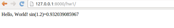
We shall start with the simplest possible application, a "scientific hello world program", where the task is to read a number and write out "Hello, World!" followed by the sine of the number. This application has one input variable and a line of text as output.
Our first implementation reads the input from the command line and writes the results to the terminal window:
#!/usr/bin/env python
import sys, math
r = float(sys.argv[1])
s = math.sin(r)
print 'Hello, World! sin(%g)=%g' % (r, s)
In the terminal we can exemplify the program
Terminal> python hw.py 1.2
Hello, World! sin(1.2)=0.932039
The task of the web version of this program is to read the r
variable from a web page, compute the sine,
and write out a new web page with the resulting text.
Before thinking of a web application, we first refactor our program
such that it fits with the classical MVC pattern and a compute component.
The refactoring does not change the functionality of the code, it
just distributes the original statements in functions and modules.
Here we create four modules: model, view,
compute, and controller.
compute module contains a function compute(r) that performs
the mathematics and returns the value s, which equals sin(r).model module holds the input data, here r.view module has two functions, one for reading input data,
get_input,
and one for presenting the output, present_output.
The latter takes the input, calls compute functionalty, and
generates the output.controller module calls the view to initialize
the model's data from the command line. Thereafter, the
view is called to present the output.model.py file contains the r variable, which must
be declared with a default value in order to create the data object:
r = 0.0    # input
s = None   # output
The view.py file is restricted to the communication with the user and reads
import sys
import compute

# Input: float r
# Output: "Hello, World! sin(r)=..."

def get_input():
    """Get input data from the command line."""
    r = float(sys.argv[1])
    return r

def present_output(r):
    """Write results to terminal window."""
    s = compute.compute(r)
    print 'Hello, World! sin(%g)=%g' % (r, s)
The mathematics is encapsulated in compute.py:
import math

def compute(r):
    return math.sin(r)
Finally, controller.py glues the model and the view:
import model, view

model.r = view.get_input()
view.present_output(model.r)
Let us try our refactored code:
Terminal> python controller.py 1.2
Hello, World! sin(1.2)=0.932039
The next step is to create a web interface to our scientific hello world
program such that we can fill in the number r in a text field, click a
Compute button and get back a new web page with the output text
shown above: "Hello, World! sin(r)=s".
Not much code or configuration is needed to make a Flask application. Actually one short file is enough. For this file to work you need to install Flask and some corresponding packages. This is easiest performed by
Terminal> sudo pip install --upgrade Flask
Terminal> sudo pip install --upgrade Flask-WTF
The --upgrade option ensures that you upgrade to the latest version in
case you already have these packages.
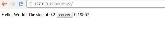
We want our input page to feature a text field where the user can
write the value of r, see Figure 1.
By clicking on the equals button
the corresponding s value is computed and written out the result page
seen in Figure 2.
Figure 1: The input page.
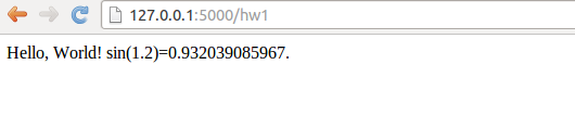
Figure 2: The output page.
Flask does not require us to use the MVC pattern so there is actually
no need to split the original program into model, view, controller,
and compute files as already explained (but it will be
done later). First we make a controller.py file where the view, the
model, and the controller parts appear within the same file.
The compute component is always in a separate file as
we like to encapsulate the computations completely from user
interfaces.
The view that the user sees is determined by
HTML templates in a subdirectory templates, and consequently
we name the template files view*.html.
The model and other parts of the view concept are just parts of
the controller.py file. The complete file is short and explained
in detail below.
from flask import Flask, render_template, request
from wtforms import Form, FloatField, validators
from compute import compute

app = Flask(__name__)

# Model
class InputForm(Form):
    r = FloatField(validators=[validators.InputRequired()])

# View
@app.route('/hw1', methods=['GET', 'POST'])
def index():
    form = InputForm(request.form)
    if request.method == 'POST' and form.validate():
        r = form.r.data
        s = compute(r)
        return render_template("view_output.html", form=form, s=s)
    else:
        return render_template("view_input.html", form=form)

if __name__ == '__main__':
    app.run(debug=True)
The web application is the app object of class Flask, and
initialized as shown. The model is a special Flask class derived from
Form where the input variable in the app is listed as a static class
attribute and initialized by a special form field object from the
wtforms package. Such form field objects correspond to HTML forms
in the input page. For the r variable we apply FloatField since
it is a floating-point variable. A default validator, here checking
that the user supplies a real number, is automatically included, but
we add another validator, InputRequired, to force the user to
provide input before clicking on the equals button.
The view part of this Python code consists of a URL and a
corresponding function to call when the URL is invoked. The function
name is here chosen to be index (inspired by the standard
index.html page that is the main page of a web app). The decorator
@app.route('/hw1', ...) maps the URL http://127.0.0.1:5000/hw1 to
a call to index. The methods argument must be as shown to allow
the user to communicate with the web page.
The index function first makes a form object based on the data in
the model, here class InputForm. Then there are two possibilities:
either the user has provided data in the HTML form or the user is
to be offered an input form. In the former case, request.method
equals 'POST' and we can extract the numerical value of r
from the form object, using form.r.data, call up our mathematical
computations, and make a web page with the result.
In the latter case, we make an input page as displayed in
Figure 1.
Making a web page with Flask is conveniently done by an HTML
template. Since the output page is simplest we display the
view_output.html template first:
Hello, World! sin({{ form.r.data }})={{s}}.
Keyword arguments sent to render_template are available in the
HTML template. Here we have the keyword arguments form and s.
With the form object we extract the value of
r in the HTML code by {{ form.r.data }}. Similarly, the value of s
is simply {{ s }}.
The HTML template for the input page is slightly more complicated as we need to use an HTML form:
<form method=post action="">
  Hello, World! The sine of {{ form.r }}
  <input type=submit value=equals>
</form>
We collect the files associated with a Flask application (often called just app) in a directory, here called hw1. All you have to do in order to run this web application is to find this directory and run
Terminal> python controller.py
 * Running on http://127.0.0.1:5000/
 * Restarting with reloader
Open a new window or tab in your browser and type in the URL
http://127.0.0.1:5000/hw1.
Our application made two distinct pages for grabbing input from the user and presenting the result. It is often more natural to add the result to the input page. This is particularly the case in the present web application, which is a kind of calculator. Figure 3 shows what the user sees after clicking the equals button.
Figure 3: The modified result page.
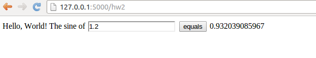
To let the user stay within the same page, we create a new directory
hw2
for this modified Flask app and copy the files from the previous
hw1 directory. The idea now is to make use of just one
template, in templates/view.html:
<form method=post action="">
  Hello, World! The sine of
  {{( form.r )}}
  <input type=submit value=equals>
{% if s != None %}
{{s}}
{% endif %}
</form>
The form is identical to what we used in view_input.html in
the hw1 directory, and the only
new thing is the output of s below the form.
The template language supports some programming with Python objects
inside {% and %} tags.
Specifically in this file, we can test on the value of s:
if it is None, we know that the computations are not performed and
s should not appear on the page, otherwise s holds the sine
value and we can write it out. Note that, contrary to plain Python,
the template language does not rely on indentation of blocks and
therefore needs an explicit end statement {% endif %} to finish
the if-test.
The generated HTML code from this template file reads
<form method=post action="">
  Hello, World! The sine of
  <input id="r" name="r" type="text" value="1.2">
  <input type=submit value=equals>

0.932039085967

</form>
The index function of our modified application
needs adjustments since we use the same
template for the input and the output page:
# View
@app.route('/hw2', methods=['GET', 'POST'])
def index():
    form = InputForm(request.form)
    if request.method == 'POST' and form.validate():
        r = form.r.data
        s = compute(r)
    else:
        s = None

    return render_template("view.html", form=form, s=s)
It is seen that if the user has given data, s is a float, otherwise
s is None. You are encouraged to test the app by running
Terminal> python controller.py
and loading http://127.0.0.1:5000/hw2 into your browser.
A nice little exercise is to control the formatting of the result s.
To this end, you can simply transform s to a string: s = '%.5f' % s before
sending it to render_template.
In our previous two Flask apps we have had the view displayed for the
user in a separate template file, and the computations as always in
compute.py, but everything else was placed in one file controller.py.
For illustration of the MVC concept we
may split the controller.py into two files: model.py and
controller.py. The view is in templates/view.html.
These new files are located in a
directory
hw3_flask
The contents
in the files reflect the splitting introduced in the original
scientific hello world program in the section Application of the MVC pattern.
The model.py file now consists of the input form class:
from wtforms import Form, FloatField, validators

class InputForm(Form):
    r = FloatField(validators=[validators.InputRequired()])
The file templates/view.html is as before, while controller.py contains
from flask import Flask, render_template, request
from compute import compute
from model import InputForm

app = Flask(__name__)

@app.route('/hw3', methods=['GET', 'POST'])
def index():
    form = InputForm(request.form)
    if request.method == 'POST' and form.validate():
        r = form.r.data
        s = compute(r)
    else:
        s = None

    return render_template("view.html", form=form, s=s)


if __name__ == '__main__':
    app.run(debug=True)
The statements are indentical to those in the hw2 app, only
the organization of the statement in files differ.
You can easily kill the Flask application and restart it, but sometimes
you will get an error that the address is already in use.
To recover from this problem, run the lsof program to see which program
that applies the 5000 port (Flask runs its server on http://127.0.0.1:5000,
which means that it uses the 5000 port). Find the PID of the program
that occupies the port and force abortion of that program:
Terminal> lsof -i :5000
COMMAND   PID USER   FD   TYPE  DEVICE SIZE/OFF NODE NAME
python  48824  hpl    3u  IPv4 1128848      0t0  TCP ...
Terminal> kill -9 48824
You are now ready to restart a Flask application.
We recommend to
download and istall the latest official version of Django from
http://www.djangoproject.com/download/. Pack out the tarfile, go
to the directory, and run setup.py:
Terminal> tar xvzf Django-1.5-tar.gz
Terminal> cd Django-1.5
Terminal> sudo python setup.py install
The version in this example, 1.5, may be different at the time you follow these instructions.
Django applies two concepts: project and application (or app). The app is the program we want to run through a web interface. The project is a Python package containing common settings and configurations for a collection of apps. This means that before we can make a Django app, we must to establish a Django project.
A Django project for managing a set of Django apps is created by the command
Terminal> django-admin.py startproject django_project
The result in this example
is a directory django_project whose content can be explored
by some ls and cd commands:
Terminal> ls django_project
manage.py django_project
Terminal> cd django_project/django_project
Terminal> ls
__init__.py settings.py urls.py wsgi.py
The meaning of the generated files is briefly listed below.
django_project/ directory is just a container for your project. Its name does not matter to Django.manage.py is a command-line utility that lets you interact with this Django project in various ways. You will typically run manage.py to launch a Django application.django_project/ directory is a Python package for the Django project. Its name is used in import statements in Python code (e.g., import django_project.settings).django_project/__init__.py is an empty file that just tells Python that this directory should be considered a Python package.django_project/settings.py contains the settings and configurations for this Django project.django_project/urls.py maps URLs to specific functions and thereby defines that actions that various URLs imply.django_project/wsgi.py is not needed in our examples.
Terminal> python manage.py runserver
Validating models...

0 errors found
March 34, 201x - 01:09:24
Django version 1.5, using settings 'django_project.settings'
Development server is running at http://127.0.0.1:8000/
Quit the server with CONTROL-C.
The output from starting the server tells that the server runs on the
URL http://127.0.0.1:8000/.
Load this URL into your browser to see a welcome message from Django,
meaning that the server is working.
Despite the fact that our introductory
web applications do not need a database, you
have to register a database with any Django project. To this end,
open the django_project/settings.py file in a text editor,
locate the DATABASES dictionary and type in the following
code:
import os

def relative2absolute_path(relative_path):
    """Return the absolute path correspodning to relative_path."""
    dir_of_this_file = os.path.dirname(os.path.abspath(__file__))
    return dir_of_this_file + '/' + relative_path

DATABASES = {
   'default' : {
      'ENGINE': 'django.db.backends.sqlite3',
      'NAME': relative2absolute_path('../database.db')
   }
}
The settings.py file needs absolute paths to files, while it is
more convenient for us to specify relative paths. Therefore,
we made a function that figures out the absolute path to the settings.py
file and then combines this absolute path with the relative path.
The location and name of the database file can be chosen as desired.
Note that one should not use os.path.join to create paths as Django
always applies the forward slash between directories, also on Windows.
The next step is to create a Django app for our scientific hello
world program. We can place the app in any directory, but here we
utilize the following organization.
As neighbor to django_project we have
a directory apps containing our various scientific applications.
Under apps we create a directory django_apps with
our different versions of Django applications.
The directory py_apps contains the
original hw.py program in the subdirectory orig,
while split of this
program according to the MVC pattern appears in the mvc directory.
The directory django_apps/hw1 is our first attempt to write
a Django-based web interface for the hw.py program.
The directory structure is laid out by
Terminal> cd ..
Terminal> mkdir apps
Terminal> cd apps
Terminal> mkdir py_apps
Terminal> cd py
Terminal> mkdir orig mvc
Terminal> cd ../..
Terminal> mkdir django_apps
Terminal> cd django_apps
The file hw.py is moved to orig while mvc contains
the MVC refactored version with the files model.py, view.py, compute.py,
and controller.py.
The hw1 directory, containing our first Django application, must be
made with
Terminal> python ../../django_project/manage.py startapp hw1
The command creates a directory hw1 with four empty files:
Terminal> cd hw1
Terminal> ls
__init__.py models.py tests.py views.py
The __init__.py file will remain empty to just indicate that the
Django application is a Python package. The other files need to be
filled with the right content, which happens in the next section.
At this point,
we need to register some information about our application in the
django_project/settings.py and django_project/urls.py files.
Step 1: Add the app.
Locate the INSTALLED_APPS
tuple in settings.py and add your Django application as a Python package:
INSTALLED_APPS = (
    'django.contrib.auth',
    'django.contrib.contenttypes',
    ...
    'hw1',
)
Unfortunately, Django will not be able to find the package hw1
unless we register the parent directory in sys.path:
import sys
sys.path.insert(0, relative2absolute_path('../../apps/django_apps'))
Note here that the relative path is given with respect to the
location of the settings.py script.
Step 2: Add a template directory.
Make a subdirectory templates under hw1,
Terminal> mkdir templates
and add the absolute path of this directory to the TEMPLATE_DIRS tuple:
TEMPLATE_DIRS = (
    relative2absolute_path('../../apps/django_apps/hw1/templates'),
)
The templates directory will hold templates for the HTML code applied
in the web interfaces. The trailing comma is important as this is
a tuple with only one element.
Step 3: Define the URL.
We need to connect the Django app with
an URL. Our app will be associated with a Python function index
in the views module within the hw1 package.
Say we want the corresponding URL to
be named hw1 relative to the server URL.
This information is registered in the django_project/urls.py file
by the syntax
urlpatterns = patterns('',
    url(r'^hw1/', 'django_apps.hw1.views.index'),
The first argument to the url function is a regular expression for
the URL and the second argument is the name of the function to call,
using Python's syntax for a function index in a module views in
a package hw1.
The function name index resembles the index.html main page associated
with an URL, but any other name than index can be used.
The Django application is about filling the files views.py and models.py
with content. The mathematical computations are performed in compute.py
so we copy this file from the mvc directory to the hw1 directory
for convenience (we could alternatively add ../mvc to sys.path such that
import compute would work from the hw1 directory).
The web application offers a text field where the user can
write the value of r, see Figure 4.
After clicking on the equals button,
the mathematics is performed and a new page as
seen in Figure 5 appears.
Figure 4: The input page.
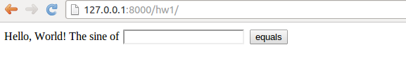
Figure 5: The result page.
The models.py file contains the model, which consists
of the data we need in the application, stored in Django's data types.
Our data consists of one number, called r, and models.py then
look like
from django.db import models
from django.forms import ModelForm

class Input(models.Model):
    r = models.FloatField()

class InputForm(ModelForm):
    class Meta:
        model = Input
The Input class lists variables representing data as static class
attributes. The django.db.models module contains various classes
for different types of data, here we use FloatField to represent
a floating-point number.
The InputForm class has a the shown generic form across applications
if we by convention apply the name Input for the class holding the data.
The views.py file contains a function index which defines
the actions we want to perform when invoking
the URL ( here http://127.0.0.1:8000/hw1/).
In addition, views.py has the present_output function from
the view.py file in the mvc directory.
from django.shortcuts import render_to_response
from django.template import RequestContext
from django.http import HttpResponse
from models import InputForm
from compute import compute

def index(request):
    if request.method == 'POST':
        form = InputForm(request.POST)
        if form.is_valid():
            form = form.save(commit=False)
            return present_output(form)
    else:
        form = InputForm()

    return render_to_response('hw1.html',
            {'form': form}, context_instance=RequestContext(request))

def present_output(form):
    r = form.r
    s = compute(r)
    return HttpResponse('Hello, World! sin(%s)=%s' % (r, s))
The index function deserves some explanation. It must take one
argument, usually called request. There are two modes in the function. Either
the user has provided input on the web page, which means that
request.method equals 'POST', or we show a new web page
with which the user is supposed to interact.
The input consists of a web form with
one field where we can fill in our r variable. This page
is realized by the two central statements
# Make info needed in the web form
form = InputForm()
# Make HTML code
render_to_response('hw1.html',
    {'form': form}, context_instance=RequestContext(request))
The hw1.html file resides in the templates subdirectory and contains
a template for the HTML code:
<form method="post" action="">{% csrf_token %}
    Hello, World! The sine of {{ form.r }}
    <input type="submit" value="equals" />
</form>
This is a template file because it contains instructions like
{% csrf_token %} and variables like {{ form.r }}. Django will
replace the former by some appropriate HTML statements, while the
latter simply extracts the numerical value of the variable r in
our form (specified in the Input class in models.py).
Typically, this hw1.html file
results in the HTML code
<form method="post" action="">
<div style='display:none'>
<input type='hidden' name='csrfmiddlewaretoken'
value='oPWMuuy1gLlXm9GvUZINv49eVUYnux5Q' /></div>
    Hello, World! The sine of <input type="text" name="r" id="id_r" />
    <input type="submit" value="equals" />
</form>
When then user has filled in a value in the text field on the input
page, the index function is called again and request.method equals
'POST'. A new form object is made, this time with user info (request.POST).
We can check that the form is valid and if so, proceed with
computations followed by presenting the results in a
new web page (see Figure 5):
def index(request):
    if request.method == 'POST':
        form = InputForm(request.POST)
        if form.is_valid():
            form = form.save(commit=False)
            return present_output(form)

def present_output(form):
    r = form.r
    s = compute(r)
    return HttpResponse('Hello, World! sin(%s)=%s' % (r, s))
The numerical value of r as given by the user is available as form.r.
Instead of using a template for the output page, which is natural to
do in more advanced cases, we here illustrate the possibility to
send raw HTML to the output page by returning an HttpResponse
object initialized by a string containing the desired HTML code.
Launch this application by filling in the address http://127.0.0.1:8000/hw1/
in your web browser. Make sure the Django development server is running,
and if not, restart it by
Terminal> python ../../../django_project/manage.py runserver
Fill
in some number on the input page and view the output.
To show how easy it is to change the application, invoke the views.py
file in an editor and add some color to the output HTML code from
the present_output function:
    return HttpResponse("""
<font color='blue'>Hello</font>, World!
sin(%s)=%s
"""% (r, s))
Go back to the input page, provide a new number, and observe how the "Hello" word now has a blue color.
Instead of making a separate output page with the result, we can simply add the sine value to the input page. This makes the user feel that she interacts with the same page, as when operating a calculator. The output page should then look as shown in Figure 6.
Figure 6: The modified result page.
We need to make a new Django application, now called
hw2.
Instead of running the standard
manage.py startapp hw2 command,
we can simply copy the hw1
directory to hw2. We need, of course, to add information about this
new application in settings.py and urls.py.
In the former file we must have
TEMPLATE_DIRS = (
    relative2absolute_path('../../apps/django_apps/hw1/templates'),
    relative2absolute_path('../../apps/django_apps/hw2/templates'),
)

INSTALLED_APPS = (
    'django.contrib.auth',
    'django.contrib.contenttypes',
    'django.contrib.sessions',
    'django.contrib.sites',
    'django.contrib.messages',
    'django.contrib.staticfiles',
    # Uncomment the next line to enable the admin:
    # 'django.contrib.admin',
    # Uncomment the next line to enable admin documentation:
    # 'django.contrib.admindocs',
    'hw1',
    'hw2',
)
In urls.py we add the URL hw2 which is to call our index function
in the views.py file of the hw2 app:
urlpatterns = patterns('',
    url(r'^hw1/', 'django_apps.hw1.views.index'),
    url(r'^hw2/', 'django_apps.hw2.views.index'),
The views.py file changes a bit since we shall generate almost the same
web page on input and output. This makes the present_output function
unnatural, and everything is done within the index function:
def index(request):
    s = None  # initial value of result
    if request.method == 'POST':
        form = InputForm(request.POST)
        if form.is_valid():
            form = form.save(commit=False)
            r = form.r
            s = compute(r)
    else:
        form = InputForm()

    return render_to_response('hw2.html',
            {'form': form,
             's': '%.5f' % s if isinstance(s, float) else ''
             }, context_instance=RequestContext(request))
Note that the output variable s is computed within the index
function and defaults to None. The template file hw2.html
looks like
<form method="post" action="">{% csrf_token %}
    Hello, World! The sine of {{ form.r }}
    <input type="submit" value="equals" />
{% if s != '' %}
{{ s }}
{% endif %}
</form>
The difference from hw1.html is that we right after the equals
button write out the value of s. However, we make a test that
the value is only written if it is computed, here recognized by
being a non-empty string. The s in the template file
is substituted by the value of the object
corresponding to the key 's' in the
dictionary we pass to the render_to_response. As seen,
we pass a string where s is formatted with five digits if s
is a float, i.e., if s is computed. Otherwise, s has the
default value None and we send an empty string to the template.
The template language allows tests using Python syntax, but the
if-block must be explicitly ended by {% endif %}.
The scientific hello world example shows how to work with one input
variable and one output variable. We can easily derive an extensible
recipe for apps with a collection of input variables and some
associated HTML code as result. Multiple input variables are listed
in the InputForm class using different types for different forms
(text field, float field, integer field, check box field for boolean
values, etc.). The value of these variables will be available in a
form object for computation. It is then a matter of setting
up a template code where the various variables if the form object
are formatted in HTML code as desired.
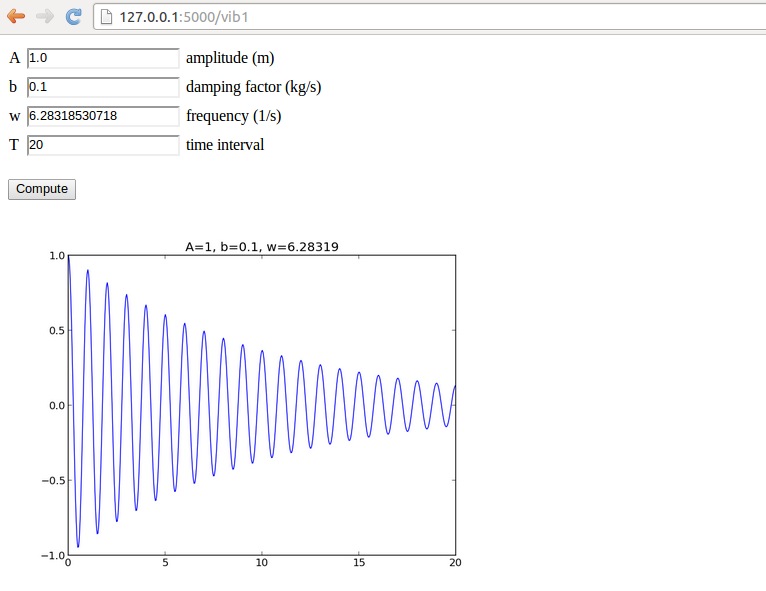
Our sample web application addresses the task of plotting the function \( u(t)=Ae^{-bt}\sin (wt) \) for \( t\in [0,T] \). The web application must have fields for the numbers \( A \), \( b \), \( w \), and \( T \), and a Compute button, as shown in Figure 7. Filling in values, say \( 0.1 \) for \( b \) and \( 20 \) for \( T \), results in what we see in Figure 8, i.e., a plot of \( u(t) \) is added after the input fields and the Compute button.
Figure 7: The input page.
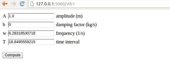
Figure 8: The result page.
We shall make a series of different versions of this app:
vib1 for the basic set-up and illustration of tailoring the HTML code.vib2 for custom validation of input, governed by the programmer,
and inlined graphics in the HTML code.vib3 for interactive Bokeh plots.gen for automatic generation of the Flask app (!).login for storing computed results in user accounts.upload for uploading files to a web app.
The forthcoming text explains the necessary steps to realize a
Flask app that behaves as depicted in Figures 7
and 8. We start with the
compute.py module since it contains only the computation of \( u(t) \)
and the making of the plot, without any interaction with Flask.
The files associated with this app are found in the vib1 directory.
More specifically, inside compute.py, we have a function for
evaluating \( u(t) \) and a compute function for making the plot. The
return value of the latter is the name of the plot file, which should
get a unique name every time the compute function is called such
that the browser cannot reuse an already cached image when displaying
the plot. Flask
applications must have all extra files (CSS, images, etc.) in a
subdirectory static.
from numpy import exp, cos, linspace
import matplotlib.pyplot as plt
import os, time, glob

def damped_vibrations(t, A, b, w):
    return A*exp(-b*t)*cos(w*t)

def compute(A, b, w, T, resolution=500):
    """Return filename of plot of the damped_vibration function."""
    t = linspace(0, T, resolution+1)
    u = damped_vibrations(t, A, b, w)
    plt.figure()  # needed to avoid adding curves in plot
    plt.plot(t, u)
    plt.title('A=%g, b=%g, w=%g' % (A, b, w))
    if not os.path.isdir('static'):
        os.mkdir('static')
    else:
        # Remove old plot files
        for filename in glob.glob(os.path.join('static', '*.png')):
            os.remove(filename)
    # Use time since Jan 1, 1970 in filename in order make
    # a unique filename that the browser has not chached
    plotfile = os.path.join('static', str(time.time()) + '.png')
    plt.savefig(plotfile)
    return plotfile

if __name__ == '__main__':
    print compute(1, 0.1, 1, 20)
It is in general not a good idea to write plots to file or let a
web app write to file. If this app is deployed at some web site and
multiple users are running the app, the os.remove statements may remove
plots created by all other users. However, the app is useful as a
graphical user interface run locally on a machine.
Later, we shall avoid writing plot files and instead
store plots in strings and embed the strings
in the img tag in the HTML code.
We organize the model, view, and controller as three separate files, as illustrated in the section Splitting the app into model, view, and controller files. This more complicated app involves more code and especially the model will soon be handy to isolate in its own file.
Our first version of model.py reads
from wtforms import Form, FloatField, validators
from math import pi

class InputForm(Form):
    A = FloatField(
        label='amplitude (m)', default=1.0,
        validators=[validators.InputRequired()])
    b = FloatField(
        label='damping factor (kg/s)', default=0,
        validators=[validators.InputRequired()])
    w = FloatField(
        label='frequency (1/s)', default=2*pi,
        validators=[validators.InputRequired()])
    T = FloatField(
        label='time interval (s)', default=18,
        validators=[validators.InputRequired()])
As seen, the field classes can take a label argument for a longer
description, here also including the units in which the variable is
measured. It is also possible to add a description argument with
some help message. Furthermore, we include a default value, which
will appear in the text field such that the user does not need to
fill in all values.
The view component will of course make use of templates, and we shall experiment
with different templates. Therefore, we allow a command-line argument
to this Flask app for choosing which template we want. The rest of
the controller.py file follows much the same set up as for the scientific
hello world app:
from model import InputForm
from flask import Flask, render_template, request
from compute import compute

app = Flask(__name__)

@app.route('/vib1', methods=['GET', 'POST'])
def index():
    form = InputForm(request.form)
    if request.method == 'POST' and form.validate():
        result = compute(form.A.data, form.b.data,
                         form.w.data, form.T.data)
    else:
        result = None

    return render_template('view.html', form=form, result=result)

if __name__ == '__main__':
    app.run(debug=True)
The details governing how the web page really looks like lie in the
template file. Since we have several fields and want them nicely
align in a tabular fashion, we place the field name, text areas,
and labels inside an HTML table in our first attempt to write a
template, view_plain.html:
<form method=post action="">
<table>
  {% for field in form %}
    <tr>
    <td>{{ field.name }}</td><td>{{ field }}</td>
    <td>{{ field.label }}</td>
    </tr>
  {% endfor %}
</table>
<p><input type=submit value=Compute></form></p>

<p>
{% if result != None %}
<img src="{{ result }}" width="500">
{% endif %}
</p>
Observe how easy it is to iterate over the form object and grab data
for each field: field.name is the name of the variable in the
InputForm class, field.label is the full name with units as given
through the label keyword when constructing the field object, and
writing the field object itself generates the text area for
input (i.e., the HTML input form). The control statements we can
use in the template are part of the Jinja2
templating language. For now, the if-test, for-loop and
output of values ({{ object }}) are enough to generate the HTML
code we want.
Recall that the objects we need in the template, like result and form
in the present case, are transferred to the template via keyword
arguments to the render_template function. We can easily pass on
any object in our application to the template. Debugging of the template
is done by viewing the HTML source of the web page in the browser.
You are encouraged to go to the vib1 directory,
run python controller.py, and load
`http://127.0.0.1:5000/vib1`
into your web browser for testing.
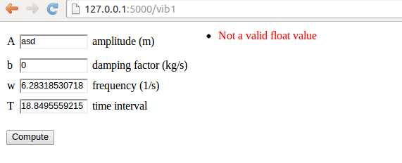
What happens if the user gives wrong input, for instance the letters asd
instead of a number? Actually nothing! The FloatField object
checks that the input is compatible with a real number in the
form.validate() call, but returns just False if this is not
the case. Looking at the code in controller.py,
def index():
    form = InputForm(request.form)
    if request.method == 'POST' and form.validate():
        result = compute(form.A.data, form.b.data,
                         form.w.data, form.T.data)
    else:
        result = None
we realize that wrong input implies result = None and no computations
and no plot! Fortunately, each field object gets an attribute error
with information on errors that occur on input. We can write out
this information on the web page, as exemplified in the template
view_errcheck.html:
<form method=post action="">
<table>
  {% for field in form %}
    <tr>
    <td>{{ field.name }}</td><td>{{ field(size=12) }}</td>
    <td>{{ field.label }}</td>
    {% if field.errors %}
      <td><ul class=errors>
      {% for error in field.errors %}
        <li><font color="red">{{ error }}</font></li>
      {% endfor %}</ul></td>
    {% endif %}
    </tr>
  {% endfor %}
</table>
<p><input type=submit value=Compute></form></p>
<p>
{% if result != None %}
<img src="{{ result }}" width="500">
{% endif %}
</p>
Two things are worth noticing here:
A field by
writing asd instead of a number. This input
triggers an error, whose message is written in red to the right of the label,
see Figure 9.
Figure 9: Error message because of wrong input.
It is possible to use the additional HTML5 fields for input in a Flask context. Instead of explaining how here, we recommend to use the Parampool package to automatically generate Flask files with HTML5 fields.
Web developers make heavy use of CSS style sheets to control the look
and feel of web pages. Templates can utilize style sheets as any other
standard HTML code. Here is a very simple example where we introduce
a class name for the HTML table's column with the field name and set the
foreground color of the text in this column to blue.
The style sheet is called basic.css and must reside in the
static subdirectory of the Flask application directory. The content
of basic.css is just the line
td.name { color: blue; }
The view_css.html file using this style sheet features a link tag
to the style sheet in the HTML header, and the column containing
the field name has
the HTML tag <td class="name"> to trigger the specification in
the style sheet:
<html>
<head>
<link rel="stylesheet" href="static/basic.css" type="text/css">
</head>
<body>

<form method=post action="">
<table>
  {% for field in form %}
    <tr>
    <td class="name">{{ field.name }}</td>
    <td>{{ field(size=12) }}</td>
    <td>{{ field.label }}</td>
Just run python controller.py view_css to see that the names
of the variables to set in the web page are blue.
Scientific applications frequently have many input data that are
defined through mathematics and where the typesetting on the
web page should be as close as possible to the typesetting where
the mathematics is documented. In the present example we would like
to typeset \( A \), \( b \), \( w \), and \( T \) with italic font as done
in LaTeX. Fortunately, native LaTeX typesetting is available in
HTML through the tool MathJax.
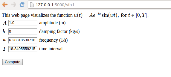
Our template view_tex.html enables MathJax. Formulas are written
with standard LaTeX inside \( and \), while equations are surrounded
by $$. Here we use formulas only:
<script type="text/x-mathjax-config">
MathJax.Hub.Config({
  TeX: {
     equationNumbers: {  autoNumber: "AMS"  },
     extensions: ["AMSmath.js", "AMSsymbols.js", "autobold.js", "color.js"]
  }
});
</script>
<script type="text/javascript"
 src="http://cdn.mathjax.org/mathjax/latest/MathJax.js?config=TeX-AMS-MML_HTMLorMML">
</script>

This web page visualizes the function \(
u(t) = Ae^{-bt}\sin (w t), \hbox{ for } t\in [0,T]
\).

<form method=post action="">
<table>
  {% for field in form %}
    <tr>
    <td>\( {{ field.name }} \)</td><td>{{ field(size=12) }}</td>
    <td>{{ field.label }}</td>
Figure 10 displays how the LaTeX rendering looks like in the browser.
Figure 10: LaTeX typesetting of mathematical symbols.
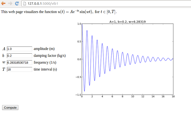
Now we want to place the plot to the right of the input forms in the web page, see Figure 11. This can be accomplished by having an outer table with two rows. The first row contains the table with the input forms in the first column and the plot in the second column, while the second row features the Compute button in the first column.
Figure 11: New design with input and output side by side.
The enabling template file is view_table.html:
<script type="text/x-mathjax-config">
MathJax.Hub.Config({
  TeX: {
     equationNumbers: {  autoNumber: "AMS"  },
     extensions: ["AMSmath.js", "AMSsymbols.js", "autobold.js"]
  }
});
</script>
<script type="text/javascript"
 src="http://cdn.mathjax.org/mathjax/latest/MathJax.js?config=TeX-AMS-MML_HTMLorMML">
</script>

This web page visualizes the function \(
u(t) = Ae^{-bt}\sin (w t), \hbox{ for } t\in [0,T]
\).

<form method=post action="">
<table> <!-- table with forms to the left and plot to the right -->
<tr><td>
<table>
  {% for field in form %}
    <tr>
    <td>\( {{ field.name }} \)</td><td>{{ field(size=12) }}</td>
    <td>{{ field.label }}</td>
    {% if field.errors %}
      <td><ul class=errors>
      {% for error in field.errors %}
        <li><font color="red">{{ error }}</font></li>
      {% endfor %}</ul></td>
    {% endif %}
    </tr>
  {% endfor %}
</table>
</td>

<td>
<p>
{% if result != None %}
<img src="{{ result }}" width="500">
{% endif %}
</p>
</td></tr>
<tr>
<td><p><input type=submit value=Compute></p></td>
</tr>
</table>
</form>
The Bootstrap framework for creating web pages
has been very popular in recent years, both because of the design and
the automatic support for responsive pages on all sorts of devices.
Bootstrap can easily be used in combination with Flask. The template file
view_bootstrap.html is identical to the former view_table.html,
except that we load the Bootstrap CSS file and include in comments
how to add the typical navigation bar found in many Bootstrap-based
web pages. Moreover, we use the grid layout functionality of Bootstrap
to control the placement of elements (name, input field, label,
and error message) in the input form.
The template looks like
<!DOCTYPE html>
<html lang="en">
<link href=
"http://netdna.bootstrapcdn.com/bootstrap/3.1.1/css/bootstrap.min.css"
rel="stylesheet">
<script type="text/x-mathjax-config">
MathJax.Hub.Config({
TeX: {
equationNumbers: { autoNumber: "AMS" },
extensions: ["AMSmath.js", "AMSsymbols.js", "autobold.js", "color.js"]
}
});
</script>
<script type="text/javascript" src=
"http://cdn.mathjax.org/mathjax/latest/MathJax.js?config=TeX-AMS-MML_HTMLorMML">
</script>
<!--
<nav class="navbar navbar-default" role="navigation">
<div class="collapse navbar-collapse" id="bs-example-navbar-collapse-1">
<ul class="nav navbar-nav">
{% for text, url in some_sequence %}
<li><a href="/{{url}}">{{ text }}</a></li>
{% endfor %}
</ul>
</div>
</nav>
-->
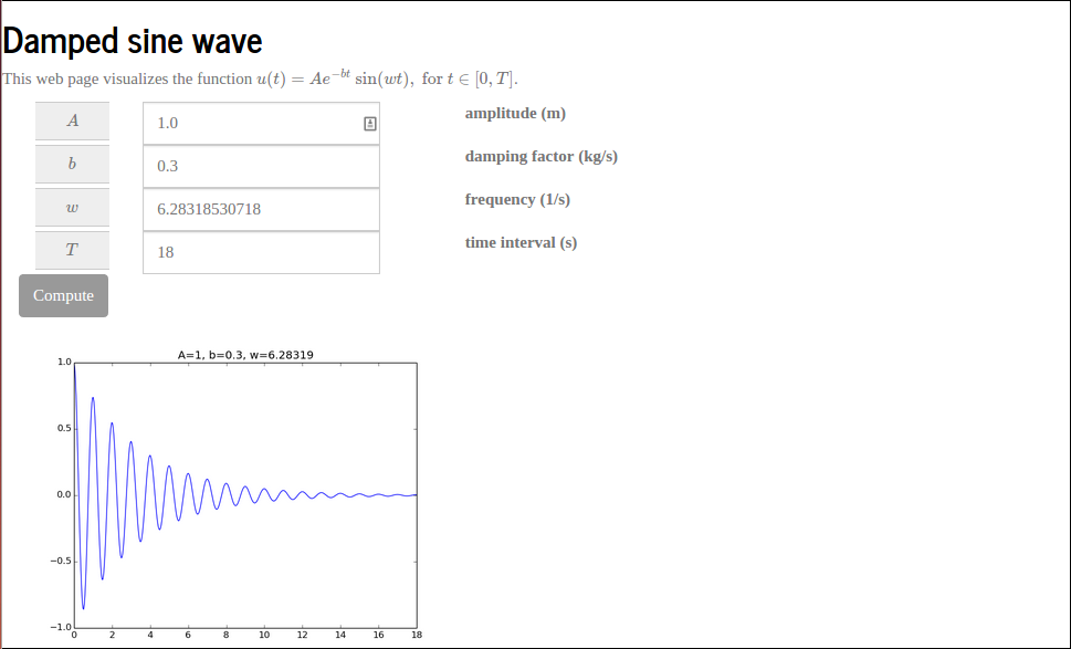
<h2>Damped sine wave</h2>
This web page visualizes the function \(
u(t) = Ae^{-bt}\sin (w t), \hbox{ for } t\in [0,T]
\).
<p>
<form class="navbar-form navbar-top" method="post" action="">
<div class="form-group">
{% for field in form %}
<div class="row">
<div class="input-group">
<label class="col-xs-1 control-label">
<span class="input-group-addon"> \( {{ field.name }} \) </span>
</label>
<div class="col-xs-2">
{{ field(class_="form-control") }}
</div>
<div class="col-xs-3">
{{ field.label }}
</div>
{% if field.errors %}
{% for error in field.errors %}
<div class="col-xs-3">
<div style="color: red;">{{ error }}</div>
</div>
{% endfor %}
{% endif %}
</div>
</div>
{% endfor %}
<br/>
<input type="submit" value="Compute" class="btn btn-default">
</form>
<p>
{% if result != None %}
<img src="{{ result }}" width="400">
{% endif %}
</html>
The input fields and fonts now get the typical Bootstrap look and feel:
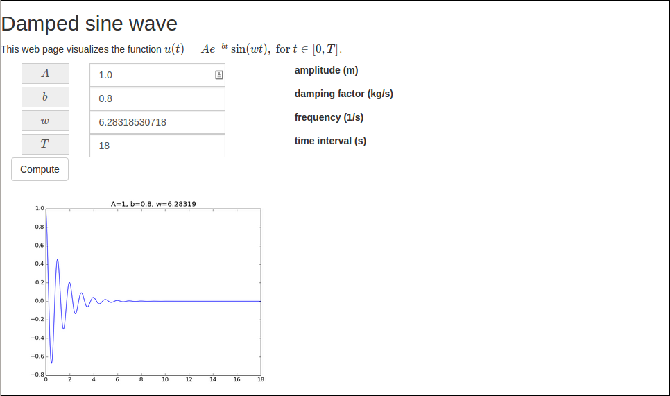
The only special feature in this template is the need to pass a CSS
class form-control to the field object in the part that defines
the input field. We also use the standard input-group-addon style
in the name part of the Bootstrap form. A heading Damped sine wave was
added to demonstrate the Bootstrap fonts.
It is easy to switch to other Bootstrap styles, e.g., those in the "Bootswatch family": "http:bootswatch.com":
<link href=
"http://netdna.bootstrapcdn.com/bootswatch/3.1.1/X/bootstrap.min.css"
rel="stylesheet">
where X can be journal, cosmo, flatly, and other legal
Bootswatch styles. The journal style looks like this:
While view_bootstrap.html makes use of plain Bootstrap HTML code, there is
also a higher-level framework, called Flask-Bootstrap that combines Flask and Bootstrap. Installation of
this extension is done by sudo pip install flask-bootstrap.
After app = Flask(__name__) we need to do
from flask_bootstrap import Bootstrap
Bootstrap(app)
We introduce a command-line argument to control whether we want the
plain view or the Bootstrap view. The complete controller.py file
then looks like
from model import InputForm
from flask import Flask, render_template, request
from compute import compute
import sys

app = Flask(__name__)

try:
    template_name = sys.argv[1]
except IndexError:
    template_name = 'view_plain'

if template_name == 'view_flask_bootstrap':
    from flask_bootstrap import Bootstrap
    Bootstrap(app)

@app.route('/vib1', methods=['GET', 'POST'])
def index():
    form = InputForm(request.form)
    if request.method == 'POST' and form.validate():
        result = compute(form.A.data, form.b.data,
                         form.w.data, form.T.data)
    else:
        result = None

    return render_template(template_name + '.html',
                           form=form, result=result)

if __name__ == '__main__':
    app.run(debug=True)
The template employs new keywords extends and block:
{% extends "bootstrap/base.html" %}

{% block styles %}
{{super()}}
<style>
    .appsize { width: 800px }
</style>

<script type="text/x-mathjax-config">
MathJax.Hub.Config({
  TeX: {
     equationNumbers: {  autoNumber: "AMS"  },
     extensions: ["AMSmath.js", "AMSsymbols.js", "autobold.js", "color.js"]
  }
});
</script>
<script type="text/javascript" src=
"http://cdn.mathjax.org/mathjax/latest/MathJax.js?config=TeX-AMS-MML_HTMLorMML">
</script>
{% endblock %}

<!--
{% block navbar %}
<nav class="navbar navbar-default" role="navigation">
<div class="collapse navbar-collapse" id="bs-example-navbar-collapse-1">
    <ul class="nav navbar-nav">
       {% for f in some_sequence %}
       <li><a href="/{{f}}">{{f}}</a></li>
       {% endfor %}
       </ul>
</div>
</nav>
{% endblock %}
-->

{% block content %}

<h2>Damped sine wave</h2>

This web page visualizes the function \(
u(t) = Ae^{-bt}\sin (w t), \hbox{ for } t\in [0,T]
\).

<p>
<form class="navbar-form navbar-top" method="post" action="">
  <div class="form-group">
  {% for field in form %}
    <div class="row">
     <div class="input-group appsize">
      <label class="col-sm-1 control-label">
      <span class="input-group-addon"> \( {{ field.name }} \) </span>
      </label>
      <div class="col-sm-4">
      {{ field(class_="form-control") }}
      </div>
      <div class="col-sm-4">
        {{ field.label }}
      </div>
      {% if field.errors %}
        {% for error in field.errors %}
          <div class="col-sm-3">
            <div style="color: red;">{{ error }}</div>
          </div>
        {% endfor %}
      {% endif %}
     </div>
    </div>
  {% endfor %}
<br/>
<input type="submit" value="Compute" class="btn btn-default">
</form>

<p>
{% if result != None %}
<img src="{{ result }}" width="500">
{% endif %}
</html>
{% endblock %}
It is important to have the MathJax script declaration and all styles within
{% block styles %}.
It seems easier to apply plain Bootstrap HTML code than the functionality in the Flask-Bootstrap layer.
The FloatField objects can check that the input is compatible with
a number, but what if we want to control that \( A>0 \), \( b>0 \), and
\( T \) is not greater than 30 periods (otherwise the plot gets cluttered)?
We can write functions for checking appropriate conditions and
supply the function to the list of validator functions in the call to
the FloatField constructor or other field constructors. The extra
code is a part of the model.py and the presented extensions appear
in the directory vib2.
The simplest approach to validation is to use existing functionality
in the web framework. Checking that \( A>0 \) can be done by
the NumberRange validator which checks that the value is inside
a prescribed interval:
from wtforms import Form, FloatField, validators

class InputForm(Form):
    A = FloatField(
        label='amplitude (m)', default=1.0,
        validators=[validators.NumberRange(0, 1E+20)])
We can also easily provide our own more tailored validators.
As an example, let us explain how we can check that \( T \) is less than 30 periods.
One period is \( 2\pi /w \) so we need to check if \( T> 30\cdot 2\pi/w \)
and raise an exception in that case.
A validation function takes two arguments: the whole form and the
specific field to test:
def check_T(form, field):
    """Form validation: failure if T > 30 periods."""
    w = form.w.data
    T = field.data
    period = 2*pi/w
    if T > 30*period:
        num_periods = int(round(T/period))
        raise validators.ValidationError(
            'Cannot plot as much as %d periods! T<%.2f' %
            (num_periods, 30*period))
The appropriate exception is of type validators.ValidationError.
Observe that through form we have in fact access to all the input
data so we can easily use the value of \( w \) when checking the validity
of the value of \( T \). The check_T function is easy to
add to the list of validator functions in the call to the FloatField
constructor for T:
class InputForm(Form):
    ...
    T = FloatField(
        label='time interval', default=6*pi,
        validators=[validators.InputRequired(), check_T])
The validator
objects are tested one by one as they appear in the list, and if
one fails, the others are not invoked.
We therefore add check_T after the check of input such that we know we
have a value for all data when we run the computations and test
in check_T.
Although there is already a NumberRange validator for checking
whether a value is inside an interval, we can write our own
version with some improved functionality for open intervals where
the maximum or minimum value can be infinite.
The infinite value can on input be represented by None.
A general such function may take the form
def check_interval(form, field, min_value=None, max_value=None):
    """For validation: failure if value is outside an interval."""
    failure = False
    if min_value is not None:
        if field.data < min_value:
            failure = True
    if max_value is not None:
        if field.data > max_value:
            failure = True
    if failure:
        raise validators.ValidationError(
            '%s=%s not in [%s, %s]' %
            (field.name, field.data,
             '-infty' if min_value is None else str(min_value),
             'infty'  if max_value is None else str(max_value)))
The problem is that check_interval takes four arguments, not only
the form and field arguments that a validator function in the
Flask framework can accept.
The way out of this difficulty is to use a Python tool functools.partial
which allows us to call a function with some of the arguments set beforehand.
Here, we want to create a new function that calls check_interval
with some prescribed values of min_value and max_value.
This function looks like it does not have these arguments, only
form and field. The following function produces this function, which we
can use as a valid Flask validator function:
import functools

def interval(min_value=None, max_value=None):
    return functools.partial(
        check_interval, min_value=min_value, max_value=max_value)
We can now in any field constructor just add
interval(a, b) as a validator function, here checking that \( b\in [0,\infty) \):
class InputForm(Form):
    ...
    b = FloatField(
        label='damping factor (kg/s)', default=0,
        validators=[validators.InputRequired(), interval(0,None)])
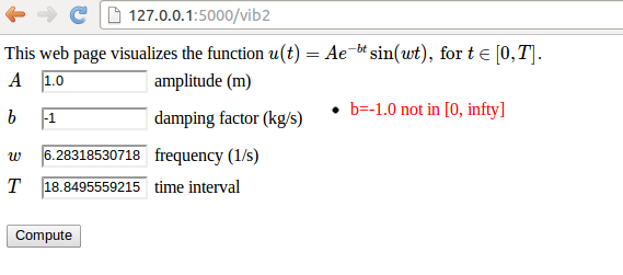
Let us test our tailored error checking. Run python controller.py
in the vib2 directory and fill in \( -1.0 \) in the \( b \) field.
Pressing Compute invokes our interval(0,None) function, which
is nothing but a call to check_interval with the
arguments field, form, 0, and None.
Inside this function,
the test if field.data < min_value becomes true, failure
is set, and the exception is raised. The message in the exception
is available in the field.errors attribute so our template
will write it out in red, see Figure 12.
The template used in vib2 is basically the same as view_tex.html
in vib1, i.e., it feaures LaTeX mathematics and checking of
field.errors.
Figure 12: Triggering of a user-defined error check.
Finally, we mention a detail in the controller.py file in the vib2
app: instead of sending form.var.data to the compute function we
may automatically generate a set of local variables such that the
application of data from the web page, here in the compute call, looks nicer:
def index():
    form = InputForm(request.form)
    if request.method == 'POST' and form.validate():
        for field in form:
            # Make local variable (name field.name)
            exec('%s = %s' % (field.name, field.data))
        result = compute(A, b, w, T)
    else:
        result = None

    return render_template(template, form=form, result=result)

if __name__ == '__main__':
    app.run(debug=True)
The idea is just to run exec on a declaration of a local variable
with name field.name for each field in the form. This trick is often
neat if web variables are buried in objects (form.T.data) and you want these
variables in your
code to look like they do in mathematical writing (T for \( T \)).
Files with plots are easy to deal with as long as they are in the
static subdirectory of the Flask application directory. However,
as already pointed out, the previous vib1 app, which writes plot
files, is not suited for multiple simultaneous users since every
user will destroy all existing plot files before making a new
one. Therefore, we need a robust solution for multiple users of
the app.
The idea is to not write plot files, but instead return the plot
as a string and embed that string directly in the HTML code.
This is relatively straightforward with Matplotlib
and Python. The relevant code is found in the compute.py file
of the vib2 app.
Python has the io.StringIO object for writing text to a
string buffer with the same syntax as used for writing text to
files. For binary streams, such as PNG files, one can use
a similar object, io.BytesIO, to hold the stream (i.e., the plot file)
in memory. The idea is to let Matplotlib write to
a io.BytesIO object and afterwards extract the
series of bytes in the plot file from this object and embed it in
the HTML file directly. This approach avoids storing plots in separate
files, at the cost of bigger HTML files.
The first step is to let Matplotlib write the PNG data to
the BytesIO buffer:
import matplotlib.pyplot as plot
from io import BytesIO
# run plt.plot, plt.title, etc.
figfile = BytesIO()
plt.savefig(figfile, format='png')
figfile.seek(0)  # rewind to beginning of file
figdata_png = figfile.getvalue()  # extract string (stream of bytes)
Before the PNG data can be embedded in HTML we need to convert the data to base64 format:
import base64
figdata_png = base64.b64encode(figdata_png)
Now we can embed the PNG data in HTML by
<img src="data:image/png;base64,PLOTSTR" width="500">
where PLOTSTR is the content of the string figdata_png.
The complete compute.py function takes the form
def compute(A, b, w, T, resolution=500):
    """Return filename of plot of the damped_vibration function."""
    t = linspace(0, T, resolution+1)
    u = damped_vibrations(t, A, b, w)
    plt.figure()  # needed to avoid adding curves in plot
    plt.plot(t, u)
    plt.title('A=%g, b=%g, w=%g' % (A, b, w))

    # Make Matplotlib write to BytesIO file object and grab
    # return the object's string
    from io import BytesIO
    figfile = BytesIO()
    plt.savefig(figfile, format='png')
    figfile.seek(0)  # rewind to beginning of file
    import base64
    figdata_png = base64.b64encode(figfile.getvalue())
    return figdata_png
The relevant syntax in an HTML template is
<img src="data:image/png;base64,{{ results }}" width="500">
if results holds the returned object from the compute function above.
Inline figures in HTML, instead of using files, are most often realized by XML code with the figure data in SVG format. Plot strings in the SVG format are created very similarly to the PNG example:
figfile = BytesIO()
plt.savefig(figfile, format='svg')
figdata_svg = figfile.getvalue()
The figdata_svg string contains XML code text can almost
be directly embedded in
HTML5. However, the beginning of the text contains information before
the svg tag that we want to remove:
<?xml version="1.0" encoding="utf-8" standalone="no"?>
<!DOCTYPE svg PUBLIC "-//W3C//DTD SVG 1.1//EN"
  "http://www.w3.org/Graphics/SVG/1.1/DTD/svg11.dtd">
<!-- Created with matplotlib (http://matplotlib.sourceforge.net/) -->
<svg height="441pt" version="1.1" viewBox="0 0 585 441" ...
The removal is done with a little string manipulation:
figdata_svg = '<svg' + figfile.getvalue().split('<svg')[1]
Now, figdata_svg can be directly inserted in HTML code without
any surrounding tags (because it is perfectly valid HTML code in itself).
The SVG code generated by Matplotlib may contain UTF-8 characters
so it is necessary to make a unicode string out of the text:
unicode(figdata_svg, 'utf-8'), otherwise the HTML template will
lead to an encoding exception.
We have made an alternative compute function compute_png_svg
that returns both a PNG and an SVG plot:
def compute_png_svg(A, b, w, T, resolution=500):
    ...
    figfile = BytesIO()
    plt.savefig(figfile, format='svg')
    figfile.seek(0)
    figdata_svg = '<svg' + figfile.getvalue().split('<svg')[1]
    figdata_svg = unicode(figdata_svg, 'utf-8')
    return figdata_png, figdata_svg
The relevant syntax for inserting an SVG plot in the HTML template is now
{{ result[1]|safe }}
The use of safe is essential here.
safe for verbatim HTML code:
Special HTML characters like <, >,
&, ", and ' are escaped in a template string like {{ str }}
(i.e., & is replaced by & `<` is replaced by <, etc.).
We need to avoid this manipulation of the string content
because result[1] contains
XML code where the mentioned characters are essential part of the syntax.
Writing {{str|safe}} ensures that the contents of the string str
are not altered before being embedded in the HTML text.
An alternative template, view_svg.html applies the SVG plot instead
of the PNG plot. We use the command-line argument svg for indicating
that we want an SVG instead of a PNG plot:
# SVG or PNG plot?
svg = False
try:
    if sys.argv[1] == 'svg':
        svg = True
except IndexError:
    pass
if svg:
    from compute import compute_png_svg as compute
    template = 'view_svg.html'
else:
    from compute import compute
    template = 'view.html'
The mpld3 library can convert Matplotlib plots to HTML code that can be directly embedded in a web page. Here is a basic example:
# Plot array y vs x
import matplotlib.pyplot as plt, mpld3
fig, ax = plt.subplots()
ax.plot(x, y)
html_text = mpld3.fig_to_html(fig)
The string html_text contains all the HTML code that is needed to
display the plot.
The great advantage of the mpld3 library is that it contains
capabilities for creating custom interactive plots through combining
Matplotlib with JavaScript, see the mpld3 Example Gallery.
As an alternative to using Matplotlib for plotting, we can utilize
the Bokeh tool, which is
particularly developed for graphics in web browsers.
The vib3 app is similar to the
previously described vib1 and vib2 app, except that we make one plot with
Bokeh. Only the compute.py and view.html files
are different. Obviously, we need to run Bokeh in the compute function.
Normally, Bokeh stores the HTML code for the plot in a file
with a specified name. We can load the text in this file and
extract the relevant HTML code for a plot. However, it is easier to
use Bokeh tools for returning the HTML code elements directly.
The steps are exemplified in the compute.py file:
from numpy import exp, cos, linspace
import bokeh.plotting as plt
import os, re

def damped_vibrations(t, A, b, w):
    return A*exp(-b*t)*cos(w*t)

def compute(A, b, w, T, resolution=500):
    """Return filename of plot of the damped_vibration function."""
    t = linspace(0, T, resolution+1)
    u = damped_vibrations(t, A, b, w)

    # create a new plot with a title and axis labels
    TOOLS = "pan,wheel_zoom,box_zoom,reset,save,box_select,lasso_select"
    p = plt.figure(title="simple line example", tools=TOOLS,
                   x_axis_label='t', y_axis_label='y')

    # add a line renderer with legend and line thickness
    p.line(t, u, legend="u(t)", line_width=2)

    from bokeh.resources import CDN
    from bokeh.embed import components
    script, div = components(p)
    head = """
<link rel="stylesheet"
 href="http://cdn.pydata.org/bokeh/release/bokeh-0.9.0.min.css"
 type="text/css" />
<script type="text/javascript"
 src="http://cdn.pydata.org/bokeh/release/bokeh-0.9.0.min.js">
</script>
<script type="text/javascript">
Bokeh.set_log_level("info");
</script>
"""
    return head, script, div
The key data returned from compute consists of a text for loading Bokeh
tools in the head part of the HTML document (common for all plots in
the file) and for the plot itself there is a script tag and a div tag. The
script tag can be placed anywhere, while the div tag must be placed
exactly where we want to have the plot. In case of multiple plots,
there will be a common script tag and one div tag for each plot.
We need to insert the three elements return from compute,
available in the tuple result, into the view.html file.
The link and scripts for Bokeh tools in result[0] is inserted
in the head part, while the script and div tags for the plot
is inserted where we want to have to plot.
The complete view.html file looks like this:
<!DOCTYPE html>
<html lang="en">
<head>
{{ result[0]|safe }}
</head>
<body>
<script type="text/x-mathjax-config">
MathJax.Hub.Config({
TeX: {
equationNumbers: { autoNumber: "AMS" },
extensions: ["AMSmath.js", "AMSsymbols.js", "autobold.js"]
}
});
</script>
<script type="text/javascript" src=
"http://cdn.mathjax.org/mathjax/latest/MathJax.js?config=TeX-AMS-MML_HTMLorMML">
</script>
This web page visualizes the function \(
u(t) = Ae^{-bt}\sin (w t), \hbox{ for } t\in [0,T]
\).
<form method=post action="">
<table>
{% for field in form %}
<tr>
<td class="name">\( {{ field.name }} \) </td>
<td>{{ field(size=12) }}</td>
<td>{{ field.label }}</td>
{% if field.errors %}
<td><ul class=errors>
{% for error in field.errors %}
<li><font color="red">{{ error }}</font></li>
{% endfor %}</ul></td>
{% endif %}
</tr>
{% endfor %}
</table>
<p><input type="submit" value="Compute"></form></p>
<p>
{% if result != None %}
<!-- script and div elements for Bokeh plot -->
{{ result[1]|safe }}
{{ result[2]|safe }}
{% endif %}
</p>
</body>
</html>
A feature of Bokeh plots is that one can zoom, pan, and save to PNG file, among other things. There is a toolbar at the top for such actions.
The controller.py file is basically the same as before (but simpler
than in the vib2 app since we do not deal with PNG and/or SVG plots):
from model import InputForm
from flask import Flask, render_template, request
from compute import compute

app = Flask(__name__)

@app.route('/vib3', methods=['GET', 'POST'])
def index():
    form = InputForm(request.form)
    if request.method == 'POST' and form.validate():
        for field in form:
            # Make local variable (name field.name)
            exec('%s = %s' % (field.name, field.data))
        result = compute(A, b, w, T)
    else:
        result = None

    return render_template('view.html', form=form,
                           result=result)

if __name__ == '__main__':
    app.run(debug=True)
Finally, we remark that Bokeh plays very well with Flask. Project 9: Interactive function exploration suggests a web app that combines Bokeh with Flask in a very interactive way.
The pandas-highcharts package is another strong alternative to Bokeh for interative plotting in web pages. It is a stable and widely used code.
We shall now present generic model.py and controller.py
files that work with any compute function (!). This example will
demonstrate some advanced, powerful features of Python. The source code
is found in the gen
directory.
The basic idea is that the Python module inspect can be used to
retrieve the names of the arguments and the default values of
keyword arguments of any given compute function. Say we have some
def mycompute(A, m=0, s=1, w=1, x_range=[-3,3]):
    ...
    return result
Running
import inspect
arg_names = inspect.getargspec(mycompute).args
defaults  = inspect.getargspec(mycompute).defaults
leads to
arg_names = ['A', 'm', 's', 'w', 'x_range']
defaults = (0, 1, 1, [-3, 3])
We have all the argument names in arg_names and
defaults[i] is the default value of keyword argument
arg_names[j], where j = len(arg_names) - len(defaults) + i.
Knowing the name name of some argument in the compute
function, we can make the corresponding class attribute
in the InputForm class by
setattr(InputForm, name, FloatForm())
For name equal to 'A' this is the same as hardcoding
class InputForm:
    A = FloatForm()
Assuming that all arguments in compute are floats, we could
do
class InputForm:
    pass  # Empty class

arg_names = inspect.getargspec(mycompute).args
for name in arg_names:
    setattr(InputForm, name, FloatForm())
However, we can do better than this: for
keyword arguments the type of the default value can be used to
select the appropriate form class. The complete model.py file
then goes as follows:
"""
Example on generic model.py file which inspects the arguments
of the compute function and automatically generates a relevant
InputForm class.
"""

import wtforms
from math import pi

from compute import compute_gamma as compute
import inspect
arg_names = inspect.getargspec(compute).args
defaults  = inspect.getargspec(compute).defaults

class InputForm(wtforms.Form):
    pass

# Augment defaults with None elements for the positional
# arguments
defaults = [None]*(len(arg_names)-len(defaults)) + list(defaults)
# Map type of default to right form field
type2form = {type(1.0): wtforms.FloatField,
             type(1):   wtforms.IntegerField,
             type(''):  wtforms.TextField,
             }

for name, value in zip(arg_names, defaults):
    if value is None:
        setattr(InputForm, name, wtforms.FloatField(
            validators=[wtforms.validators.InputRequired()]))
    else:
        if type(value) in type2form:
            setattr(InputForm, name, type2form[type(value)](
                default=value,
                validators=[wtforms.validators.InputRequired()]))
        else:
            raise TypeError('argument %s %s not supported' %
                            name, type(value))

if __name__ == '__main__':
    for item in dir(InputForm):
        if item in arg_names:
            print item, getattr(InputForm, item)
(The compute_gamma function imported from compute is the
only application-specific statement in this code and will be explained later.)
The call to compute in the controller.py file must also be expressed
in a general way such that the call handles any type and number of
parameters. This can be done in two ways, using either positional
or keyword arguments.
The technique with positional arguments
is explained first. It consists of collecting all parameters in
a list or tuple, called args, and then calling compute(*args)
(which is equivalent to compute(args[0], args[1], ..., args[n])
if n is len(args)-1). The elements of args are the values of the
form variables. We know the name of a form variable as a string
name (from arg_names), and if form is the form object,
the construction getattr(form, name).data extracts the value
that the user provided (getattr(obj, attr) gets the attribute, with name
available as a string in attr, in the object obj).
For exampe, if name is 'A', getattr(form, name).data is the same as
form.A.data.
Collecting all form variables, placing them in a list,
and calling compute are done with
arg_names = inspect.getargspec(compute).args
args = [getattr(form, name).data for name in arg_names]
result = compute(*args)
Our InputForm class guarantees that all arguments in compute
are present in the form, but to be absolutely safe we can
test if name is present in the form object:
args = [getattr(form, name).data for name in arg_names
        if hasattr(form, name)]
A potential problem with the args list is that the values might
be in wrong order. It appears, fortunately, that the order we
assign attributes to the form class is preserved when iterating over
the form. Nevertheless, using keyword arguments instead of positional
arguments provides a completely safe solution to calling compute
with the correct arguments. Keyword arguments are placed in a
dictionary kwargs and compute is called as compute(**kwargs).
The generic solution is
kwargs = {name: getattr(form, name).data for name in arg_names
          if hasattr(form, name)}
result = compute(**kwargs)
The compute(**kwargs) call is equivalent to compute(A=1, b=3, w=0.5)
in case kwargs = {'w'=0.5, 'A':1, 'b':3} (recall that the order of
the keys in a Python dictionary is undetermined).
It remains to generate the right HTML template. The HTML code depends
on what the returned result object from compute contains. Only a
human who has read the compute code knows the details of the returned
result. Therefore, we leave it to a human to provide the part
of the HTML template that renders the result. The file templates/view_results.html contains this human-provided code, while templates/view.html
is a completely generic template for the forms:
<form method=post action="">
<table>
  {% for field in form %}
    <tr><td>{{ field.name }}</td> <td>{{ field }}</td>
    <td>{% if field.errors %}
      <ul class=errors>
      {% for error in field.errors %}
        <li>{{ error }}</li>
      {% endfor %}</ul>
    {% endif %}</td></tr>
  {% endfor %}
</table>
<p><input type=submit value=Compute></form></p>

{% if result != None %}
{{ result|safe }}
{% endif %}
At the end of this code, an HTML text result (string) is to be
inserted. This text is typically generated by calling Flask's
render_template function, which uses templates/view_results.html
to turn the return object result from the compute function into the
desired HTML code:
def index():
    ...
    if result:
        result = render_template('view_results.html', result=result)
        # result is now rendered HTML text
    return render_template('view.html', form=form, result=result)
A perhaps simpler alternative would be to have a generic
view_forms.html file and a user-specific
view_results.html and explicitly combining them into a new
file. This requires file writing by the app, which one normally
wants to avoid. Especially if the web app gets multiple users,
the file writing may lead to corrupt files.
The complete, generic form of the index function becomes
def index():
    form = InputForm(request.form)
    if request.method == 'POST' and form.validate():
        arg_names = inspect.getargspec(compute).args
        kwargs = {name: getattr(form, name).data
                  for name in arg_names if hasattr(form, name)}
        result = compute(**kwargs)
    else:
        result = None
    if result:
        # result must be transformed to HTML and inserted as a
        # string in the generic view.html file
        result = render_template('view_results.html', result=result)
    return render_template('view.html', form=form, result=result)

if __name__ == '__main__':
    app.run(debug=True)
Let us apply the files above to plot the gamma probability density function
$$ g(x; a, h, A) = \frac{|h|}{\Gamma(a)A}\left(\frac{x}{A}\right)^{ah-1}
e^{-\left(\frac{x}{A}\right)^h},
$$
and its cumulative density
$$ G(x; a, h, A) = \int_0^x g(\tau; a, h, A)d\tau,$$
computed by numerically the Trapezoidal rule, for instance.
We also want to compute and display
the mean value \( A\Gamma(a + 1/h)/\Gamma(a) \) and
standard deviation
$$ \sigma = \frac{A}{\Gamma(a)}\sqrt{\Gamma(a + 2/h)\Gamma(a) - \Gamma(a+1/h)^2}.$$
Here, \( \Gamma(a) \) is the gamma function, which can be computed
by math.gamma(a) in Python.
Below is a compute.py file with the
relevant implementations of \( g(x;a,h,A) \) (gamma_density),
\( G(x; a, h, A) \) (gamma_cumulative), and a function compute_gamma for
making a plot of \( g \) og \( G \) for \( x\in [0,7\sigma] \).
def gamma_density(x, a, h, A):
    # http://en.wikipedia.org/wiki/Gamma_distribution
    xA = x/float(A)
    return abs(h)/(math.gamma(a)*A)*(xA)**(a*h-1)*exp(-xA**h)

def gamma_cumulative(x, a, h, A):
    # Integrate gamma_density using the Trapezoidal rule.
    # Assume x is array.
    g = gamma_density(x, a, h, A)
    r = zeros_like(x)
    for i in range(len(r)-1):
        r[i+1] = r[i] + 0.5*(g[i] + g[i+1])*(x[i+1] - x[i])
    return r

def compute_gamma(a=0.5, h=2.0, A=math.sqrt(2), resolution=500):
    """Return plot and mean/st.dev. value of the gamma density."""
    gah = math.gamma(a + 1./h)
    mean = A*gah/math.gamma(a)
    stdev = A/math.gamma(a)*math.sqrt(
        math.gamma(a + 2./h)*math.gamma(a) - gah**2)
    x = linspace(0, 7*stdev, resolution+1)
    y = gamma_density(x, a, h, A)
    plt.figure()  # needed to avoid adding curves in plot
    plt.plot(x, y)
    plt.title('a=%g, h=%g, A=%g' % (a, h, A))
    # Make Matplotlib write to BytesIO file object and grab
    # return the object's string
    from io import BytesIO
    figfile = BytesIO()
    plt.savefig(figfile, format='png')
    figfile.seek(0)  # rewind to beginning of file
    import base64
    figdata_density_png = base64.b64encode(figfile.getvalue())
    figfile = BytesIO()
    plt.savefig(figfile, format='svg')
    figfile.seek(0)
    figdata_density_svg = '<svg' + figfile.getvalue().split('<svg')[1]
    figdata_density_svg = unicode(figdata_density_svg,'utf-8')

    y = gamma_cumulative(x, a, h, A)
    plt.figure()
    plt.plot(x, y)
    plt.grid(True)
    figfile = BytesIO()
    plt.savefig(figfile, format='png')
    figfile.seek(0)
    figdata_cumulative_png = base64.b64encode(figfile.getvalue())
    figfile = BytesIO()
    plt.savefig(figfile, format='svg')
    figfile.seek(0)
    figdata_cumulative_svg = '<svg' + figfile.getvalue().split('<svg')[1]
    figdata_cumulative_svg = unicode(figdata_cumulative_svg,'utf-8')
    return figdata_density_png, figdata_cumulative_png, \
           figdata_density_svg, figdata_cumulative_svg, \
           '%.2f' % mean, '%.2f' % stdev
The compute_gamma function returns a tuple of six values.
We want output as displayed in Figure 13.
Figure 13: Design of a web page illustrating the gamma probability functions.
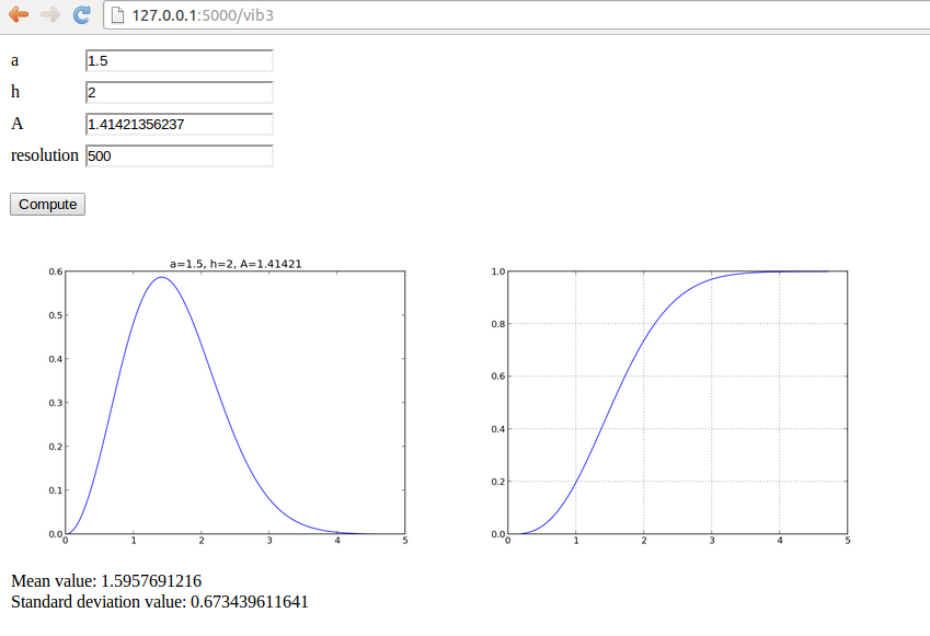
The design is realized in the file view_results.html shown below.
<p>
<table>
<tr>
<td>
<img src="data:image/png;base64,{{ result[0] }}" width="400">
</td><td>
<img src="data:image/png;base64,{{ result[1] }}" width="400">
</td></tr>
<tr>
<td>{{ result[2]|safe }}</td>
<td>{{ result[3]|safe }}</td>
</tr>
<tr><td>
Mean value: {{ result[4] }} <br>
Standard deviation value: {{ result[5] }}
</td></tr>
</table>
</p>
To create the web application, we just perform the following steps:
controller.py and model.py files to a new directorycompute.pycontroller.py and model.py to use the right name of the
compute function (from compute import name as compute)templates/view_forms.html file that visualizes
the returned value results from the compute functionWe now want to make an app where the computed results can be stored in a database. To this end, each user must create an account and login to this account for archiving results and for browsing previous runs of the application. More files are needed for this purpose, compared to the previous apps, and the files are located in the login directory.
Three more packages are needed for this more advanced application:
Installation is done by
sudo pip install --upgrade flask-login
sudo pip install --upgrade flask-sqlalchemy
sudo pip install --upgrade flask-mail
The compute.py file contains the compute
function from the vib2 app in the section Avoiding plot files.
There is quite much Flask code required for user accounts and login. The files here were generated by the Parampool package and then edited and specialized to the present application. In general, it is not recommended to hack further on the example given here, but rather utilize Parampool to generate web apps with user accounts and login.
The first page after starting the app (python controller.py)
shows input fields for the numerical parameters, but there are also
links to the right for registering a new user or logging in to an
existing account:
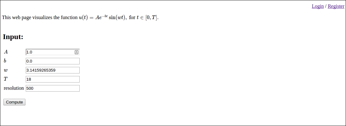
Clicking on Register brings up a registration page:
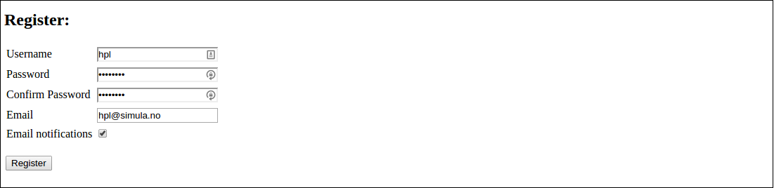
Already registered users can just log in:
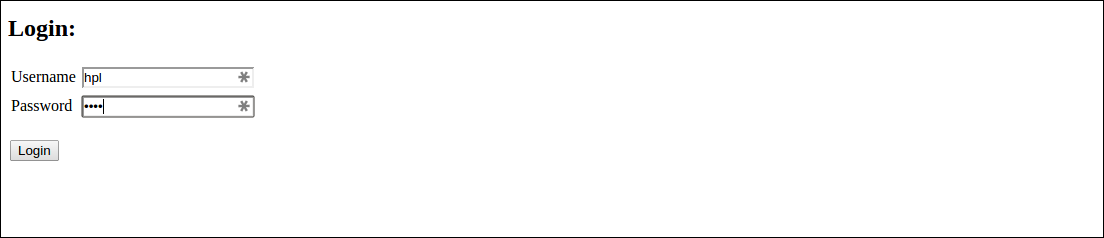
Then the fields with input parameters are shown again. After pressing Compute we are left with a combination of input and results, plus a field where the user can write a comment about this simulation:
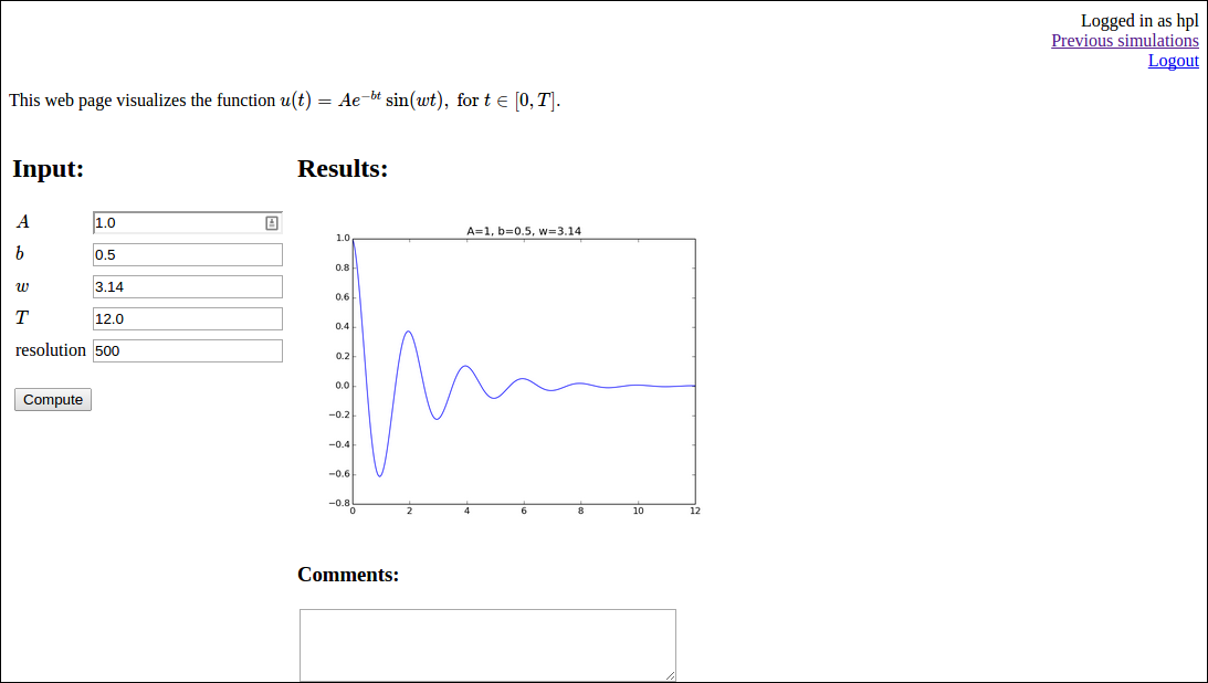
All simulations (input data, results, and comment) are stored in a database. Clicking on Previous simulation brings us to an overview of what is in the database:
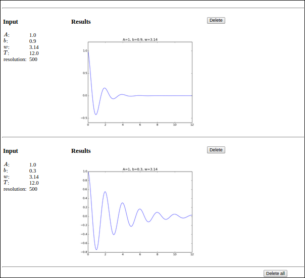
Here, one can browse previous results, remove entries, or erase the whole database.
Rather than explaining everything about the source code
in detail, we primarily list
the various code files below. A starting point is the central controller.py
file, which is now quite lengthy and involves four different
URLs (the input page, the login page, the registration page, and the
previous results page).
import os
from compute import compute as compute_function

from flask import Flask, render_template, request, redirect, url_for
from forms import ComputeForm
from db_models import db, User, Compute
from flask.ext.login import LoginManager, current_user, \
     login_user, logout_user, login_required
from app import app

login_manager = LoginManager()
login_manager.init_app(app)

@login_manager.user_loader
def load_user(user_id):
    return db.session.query(User).get(user_id)

# Path to the web application
@app.route('/', methods=['GET', 'POST'])
def index():
    result = None
    user = current_user
    form = ComputeForm(request.form)
    if request.method == "POST":
        if form.validate():

            result = compute_function(form.A.data, form.b.data,
                                      form.w.data, form.T.data)
            if user.is_authenticated():
                object = Compute()
                form.populate_obj(object)
                object.result = result
                object.user = user
                db.session.add(object)
                db.session.commit()

                # Send email notification
                if user.notify and user.email:
                    send_email(user)
    else:
        if user.is_authenticated():
            if user.Compute.count() > 0:
                instance = user.Compute.order_by('-id').first()
                result = instance.result
                form = populate_form_from_instance(instance)

    return render_template("view.html", form=form,
                           result=result, user=user)


def populate_form_from_instance(instance):
    """Repopulate form with previous values"""
    form = ComputeForm()
    for field in form:
        field.data = getattr(instance, field.name)
    return form

def send_email(user):
    from flask.ext.mail import Mail, Message
    mail = Mail(app)
    msg = Message("Compute Computations Complete",
                  recipients=[user.email])
    msg.body = """
A simulation has been completed by the Flask Compute app.
Please log in at

http://localhost:5000/login

to see the results.

---
If you don't want email notifications when a result is found,
please register a new user and leave the 'notify' field
unchecked.
"""
    mail.send(msg)

@app.route('/reg', methods=['GET', 'POST'])
def create_login():
    from forms import register_form
    form = register_form(request.form)
    if request.method == 'POST' and form.validate():
        user = User()
        form.populate_obj(user)
        user.set_password(form.password.data)

        db.session.add(user)
        db.session.commit()

        login_user(user)
        return redirect(url_for('index'))
    return render_template("reg.html", form=form)

@app.route('/login', methods=['GET', 'POST'])
def login():
    from forms import login_form
    form = login_form(request.form)
    if request.method == 'POST' and form.validate():
        user = form.get_user()
        login_user(user)
        return redirect(url_for('index'))
    return render_template("login.html", form=form)

@app.route('/logout')
@login_required
def logout():
    logout_user()
    return redirect(url_for('index'))

@app.route('/old')
@login_required
def old():
    data = []
    user = current_user
    if user.is_authenticated():
        instances = user.Compute.order_by('-id').all()
        for instance in instances:
            form = populate_form_from_instance(instance)

            result = instance.result
            if instance.comments:
                comments = "<h3>Comments</h3>" + instance.comments
            else:
                comments = ''
            data.append(
                {'form':form, 'result':result,
                 'id':instance.id, 'comments': comments})

    return render_template("old.html", data=data)

@app.route('/add_comment', methods=['GET', 'POST'])
@login_required
def add_comment():
    user = current_user
    if request.method == 'POST' and user.is_authenticated():
        instance = user.Compute.order_by('-id').first()
        instance.comments = request.form.get("comments", None)
        db.session.commit()
    return redirect(url_for('index'))

@app.route('/delete/<id>', methods=['GET', 'POST'])
@login_required
def delete_post(id):
    id = int(id)
    user = current_user
    if user.is_authenticated():
        if id == -1:
            instances = user.Compute.delete()
        else:
            try:
                instance = user.Compute.filter_by(id=id).first()
                db.session.delete(instance)
            except:
                pass

        db.session.commit()
    return redirect(url_for('old'))


if __name__ == '__main__':
    if not os.path.isfile(os.path.join(
        os.path.dirname(__file__), 'sqlite.db')):
        db.create_all()
    app.run(debug=True)
Creation of the app object is put in a separate file app.py:
import os
from flask import Flask

app = Flask(__name__)
app.config['SQLALCHEMY_DATABASE_URI'] = 'sqlite:///sqlite.db'
app.secret_key = os.urandom(24)

# Email settings
import base64
app.config.update(
        MAIL_SERVER='smtp.gmail.com',
        MAIL_PORT=587,
        MAIL_USE_TLS=True,
        MAIL_USERNAME = 'cbcwebsolvermail@gmail.com',
        MAIL_PASSWORD = base64.decodestring('WGlmZmljdox0UFch'),
        MAIL_DEFAULT_SENDER = 'Some name <name@gmail.com>'
        )
The forms for the compute function and for the login is
stored in a file called forms.py:
import wtforms as wtf
from math import pi

class ComputeForm(wtf.Form):
    A = wtf.FloatField(label='\( A \)', default=1.0,
        validators=[wtf.validators.InputRequired()])
    b = wtf.FloatField(label='\( b \)', default=0.0,
        validators=[wtf.validators.InputRequired()])
    w = wtf.FloatField(label='\( w \)', default=pi,
        validators=[wtf.validators.InputRequired()])
    T = wtf.FloatField(label='\( T \)', default=18,
        validators=[wtf.validators.InputRequired()])
    resolution = wtf.IntegerField(label='resolution', default=500,
        validators=[wtf.validators.InputRequired()])

from db_models import db, User
import flask.ext.wtf.html5 as html5

# Standard Forms
class register_form(wtf.Form):
    username = wtf.TextField(
        label='Username', validators=[wtf.validators.Required()])
    password = wtf.PasswordField(
        label='Password', validators=[
            wtf.validators.Required(),
            wtf.validators.EqualTo(
                'confirm', message='Passwords must match')])
    confirm  = wtf.PasswordField(
        label='Confirm Password',
        validators=[wtf.validators.Required()])
    email    = html5.EmailField(label='Email')
    notify   = wtf.BooleanField(label='Email notifications')

    def validate(self):
        if not wtf.Form.validate(self):
            return False

        if self.notify.data and not self.email.data:
            self.notify.errors.append(
        'Cannot send notifications without a valid email address')
            return False

        if db.session.query(User).filter_by(
            username=self.username.data).count() > 0:
            self.username.errors.append('User already exists')
            return False

        return True

class login_form(wtf.Form):
    username = wtf.TextField(
        label='Username', validators=[wtf.validators.Required()])
    password = wtf.PasswordField(
        label='Password', validators=[wtf.validators.Required()])

    def validate(self):
        if not wtf.Form.validate(self):
            return False

        user = self.get_user()

        if user is None:
            self.username.errors.append('Unknown username')
            return False

        if not user.check_password(self.password.data):
            self.password.errors.append('Invalid password')
            return False

        return True

    def get_user(self):
        return db.session.query(User).filter_by(
            username=self.username.data).first()
Database-related code for the SQLAlchemy database is collected in
db_models.py:
from flask.ext.sqlalchemy import SQLAlchemy
from werkzeug import generate_password_hash, check_password_hash
from app import app

db = SQLAlchemy(app)

class User(db.Model):
    id = db.Column(db.Integer, primary_key=True)
    username = db.Column(db.String(50), unique=True)
    pwhash = db.Column(db.String())
    email = db.Column(db.String(120), nullable=True)
    notify = db.Column(db.Boolean())

    def __repr__(self):
        return '<User %r>' % (self.username)

    def check_password(self, pw):
        return check_password_hash(self.pwhash, pw)

    def set_password(self, pw):
        self.pwhash = generate_password_hash(pw)

    def is_authenticated(self):
        return True

    def is_active(self):
        return True

    def is_anonymous(self):
        return False

    def get_id(self):
        return self.id

class Compute(db.Model):
    id = db.Column(db.Integer, primary_key=True)

    A = db.Column(db.String())
    b = db.Column(db.String())
    w = db.Column(db.String())
    T = db.Column(db.String())
    resolution = db.Column(db.Integer)

    result = db.Column(db.String())
    comments = db.Column(db.String(), nullable=True)
    user_id = db.Column(db.Integer, db.ForeignKey('user.id'))
    user = db.relationship('User',
           backref=db.backref('Compute', lazy='dynamic'))
Finally, we need views. For the results of the computation we have
a view.html file that is very similar to view_table.html
in the vib1 app:
<!DOCTYPE html>
<html lang="en">
  <head>
    <meta charset="utf-8" />
    <title>Flask Vib app</title>
  </head>
  <body>

<script type="text/x-mathjax-config">
MathJax.Hub.Config({
  TeX: {
     equationNumbers: {  autoNumber: "AMS"  },
     extensions: ["AMSmath.js", "AMSsymbols.js", "autobold.js", "color.js"]
  }
});
</script>
<script type="text/javascript" src=
"http://cdn.mathjax.org/mathjax/latest/MathJax.js?config=TeX-AMS-MML_HTMLorMML">
</script>

{% if user.is_anonymous() %}
  <p align="right"><a href="/login">Login</a>
  / <a href="/reg">Register</a></p>
{% else %}
  <p align="right">Logged in as {{user.username}}<br>
    <a href="/old">Previous simulations<a/><br>
    <a href="/logout">Logout</a></p>
{% endif %}

This web page visualizes the function \(
u(t) = Ae^{-bt}\sin (w t), \hbox{ for } t\in [0,T]
\).

<p>
<!-- Input and Results are typeset as a two-column table -->
<table>
<tr>
<td valign="top">
<h2>Input:</h2>

<form method=post action="" enctype=multipart/form-data>
<table>
  {% for field in form %}
    <tr>
      <td>{{ field.label }}</td>
      <td>{{ field(size=20) }}</td>
      <td>
      {% if field.errors %}
        <ul class=errors>
        {% for error in field.errors %}
          <li>{{ error }}</li>
        {% endfor %}</ul>
      {% endif %}
      </td></tr>
  {% endfor %}
</table>
<p>
<input type="submit" value="Compute">
</p>
</form>
</td>

<td valign="top">
  {% if result != None %}
    <h2>Results:</h2>
    <img src="data:image/png;base64,{{ result|safe }}" width="400">
    {% if not user.is_anonymous() %}
      <h3>Comments:</h3>
      <form method="post" action="/add_comment">
          <textarea name="comments" rows="4" cols="40"></textarea>
          <p><input type="submit" value="Add">
      </form>
      {% endif %}

  {% endif %}
</td></tr>
</table>
</body>
</html>
The login.html template for the login page takes the form
<!DOCTYPE html>
<html lang="en">
<head>
  <meta charset="utf-8" />
  <title>Flask Vib app</title>
</head>
<body>
<h2>Login:</h2>
<form method=post action="">
  <table>
    {% for field in form %}
      <tr><td>{{ field.label }}</td>
          <td>{{ field(size=20) }}</td>
          <td>
            {% if field.errors %}
              <ul class=errors>
              {% for error in field.errors %}
                <li>{{ error }}</li>
              {% endfor %}</ul>
            {% endif %}</td></tr>
    {% endfor %}
  </table>
  <p><input type="submit" value="Login">
</form>
</body>
</html>
The page for registering a new user has a simple template reg.html:
<!DOCTYPE html>
<html lang="en">
<head>
  <meta charset="utf-8" />
  <title>Flask Vib app</title>
</head>
<body>
<h2>Register:</h2>
<form method=post action="">
<table>
   {% for field in form %}
     <tr><td>{{ field.label }}</td>
         <td>{{ field(size=20) }}</td>
          <td>
            {% if field.errors %}
              <ul class=errors>
              {% for error in field.errors %}
                <li>{{ error }}</li>
              {% endfor %}</ul>
            {% endif %}</td></tr>
   {% endfor %}
</table>
<p><input type=submit value=Register>
</form>
</body>
</html>
The final file is old.html for retrieving old simulations:
<!DOCTYPE html>
<html lang="en">
<head>
<meta charset="utf-8" />
<title>Flask Vib app</title>
</head>
<body>
<script type="text/x-mathjax-config">
MathJax.Hub.Config({
TeX: {
equationNumbers: { autoNumber: "AMS" },
extensions: ["AMSmath.js", "AMSsymbols.js", "autobold.js", "color.js"]
}
});
</script>
<script type="text/javascript"
src="http://cdn.mathjax.org/mathjax/latest/MathJax.js?config=TeX-AMS-MML_HTMLorMML">
</script>
<h2>Previous simulations</h2>
<p align="right"><a href="/">Back to index</a></p>
{% if data %}
{% for post in data %}
<hr>
<table>
<tr>
<td valign="top" width="30%">
<h3>Input</h3>
<table>
{% for field in post.form %}
<tr><td>{{ field.label }}: </td>
<td>{{ field.data }}</td></tr>
{% endfor %}
</table>
</td><td valign="top" width="60%">
<h3>Results</h3>
<img src="data:image/png;base64,{{ post.result|safe }}" width="400">
{% if True %}
<p>
{{ comments }}
{% endif %}
</td><td valign="top" width="60%">
<p>
<form method="POST" action="/delete/{{ post.id }}">
<input type=submit value="Delete"
title="Delete this post from database">
</form>
</td></tr>
</table>
{% endfor %}
<hr>
<center>
<form method="POST" action="/delete/-1">
<input type=submit value="Delete all">
</form>
</center>
{% else %}
No previous simulations
{% endif %}
</body>
</html>
(hpl 1: Check if an autogenerated app from _generate_app.py can send mail and store comments. Need a compute function that returns full HTML text then.)
Working with a database in Flask is described here:
Many user interfaces need the user to provide data files. A minimalistic application is to have a button for uploading a single file. As example we use a file with a series of numbers, and the application's purpose is to compute the mean and standard deviation of the numbers. The first user interface just has the Choose File and Compute buttons:
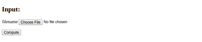
Clicking on Choose File brings up a file browser where the user can
choose the file to uploaded to the application. Say this is a file
testfile.dat. The interface now looks like
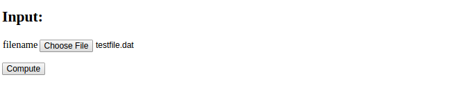
Pressing thereafter Compute leads to storage of
testfile.dat on the server in a subdirectory uploads and
computation of basic statistics of the numbers in the file.
The resulting output looks like
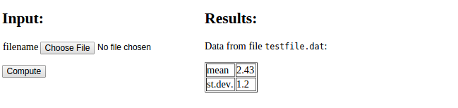
The text "No file chosen" is automatically displayed by the widget object used for file upload and indicates that a new file can be chosen. Below we shall present all parts of the code needed to create this interactive application.
The widget FieldField is used for an input field with a Choose File
button:
import wtforms as wtf

class Average(wtf.Form):
    filename   = wtf.FileField(validators=
                               [wtf.validators.InputRequired()])
The controller file needs some special code to specify a directory to store uploaded files. We also include some code to check that the file has a name with the right extension.
# Relative path of directory for uploaded files
UPLOAD_DIR = 'uploads/'

app.config['UPLOAD_FOLDER'] = UPLOAD_DIR
app.secret_key = 'MySecretKey'

if not os.path.isdir(UPLOAD_DIR):
    os.mkdir(UPLOAD_DIR)

# Allowed file types for file upload
ALLOWED_EXTENSIONS = set(['txt', 'dat', 'npy'])

def allowed_file(filename):
    """Does filename have the right extension?"""
    return '.' in filename and \
           filename.rsplit('.', 1)[1] in ALLOWED_EXTENSIONS
The index function must have code for saving the file, and as usual,
calling the compute function and rendering a new page:
def index():
    form = Average(request.form)
    filename = None  # default
    if request.method == 'POST':

        # Save uploaded file on server if it exists and is valid
        if request.files:
            file = request.files[form.filename.name]
            if file and allowed_file(file.filename):
                # Make a valid version of filename for any file ystem
                filename = secure_filename(file.filename)
                file.save(os.path.join(app.config['UPLOAD_FOLDER'],
                                       filename))

        result = compute_function(filename)
    else:
        result = None

    return render_template("view.html", form=form, result=result)
We assume that the uploaded file is available in the uploads
subdirectory, so the compute function needs to open this file, read
the numbers, and compute statistics. The file reading and computations
are easily done by numpy functions. The results are presented in
an HTML table.
import numpy as np
import os

def compute_mean_std(filename=None):
    data = np.loadtxt(os.path.join('uploads', filename))
    return """
Data from file <tt>%s</tt>:
<p>
<table border=1>
<tr><td> mean    </td><td> %.3g </td></tr>
<tr><td> st.dev. </td><td> %.3g </td></tr>
""" % (filename, np.mean(data), np.std(data))
Although the present minimalistic application only needs a very simple HTML template, we reuse a quite generic template known from previous examples, where the input variables are listed to the left and the output of the compute function is presented to the right. Such a template looks like
<!DOCTYPE html>
<html>
  <head>
    <meta charset="utf-8" />
    <title>Flask Average app</title>
  </head>
  <body>

  <!-- Input and Results are typeset as a two-column table -->
  <table>
  <tr>
  <td valign="top">
    <h2>Input:</h2>

      <form method=post action="" enctype="multipart/form-data">
        <table>
          {% for field in form %}
            <tr><td>{{ field.name }}</td>
                <td>{{ field(size=20) }}</td>
                <td>{% if field.errors %}
                  <ul class=errors>
                  {% for error in field.errors %}
                    <li>{{ error }}</li>
                  {% endfor %}</ul>
                {% endif %}</td></tr>
          {% endfor %}
        </table>
        <p><input type="submit" value="Compute">
    </form></p>
  </td>

  <td valign="top">
    {% if result != None %}
      <h2>Results:</h2>
        {{ result|safe }}

    {% endif %}
  </td>
  </tr>
  </table>
  </body>
</html>
The complete set of files is found in the upload directory.
We shall briefly how to work with multi-variable input in Django.
The text is the Django counterpart to the section Handling multiple input variables in Flask.
There are four float input variables: \( A \), \( b \), \( w \), and \( T \).
A function compute in the file compute.py makes
a plot of the function \( u(t)=Ae^{-bt}\sin (wt) \)
depending on these four parameters and returns
the name of the plot file. Our task is to define four input fields,
execute the compute function and show the input fields together with
the resulting plot,
cf. Figures 7
and 8.
Any Django app needs a project, but here we reuse the project
we set up for the scientific hello world examples. We go to
the directory apps/django_apps and create the Django app vib1:
Terminal> python ../../django_project/manage.py startapp vib1
Then we
relative2absolute_path('../../apps/django_apps/vib1/templates'),
to the TEMPLATE_DIRS tuple in settings.py,vib1 to the INSTALLED_APPS tuple, andurl(r'^vib1/', 'django_apps.vib1.views.index') to the patterns
call in urls.py.vib1 to reach the application.
The computations in our application are put in a file compute.py
and explained in detail in the section Programming the Flask application.
We can equally well utilize the Bokeh library for plotting using
the code shown in the section Plotting with the Bokeh library.
We can now write models.py and the Input class that defines
the form fields for the four input variables:
from django.db import models
from django.forms import ModelForm
from math import pi

class Input(models.Model):
    A = models.FloatField(
        verbose_name=' amplitude (m)', default=1.0)
    b = models.FloatField(
        verbose_name=' damping coefficient (kg/s)', default=0.0)
    w = models.FloatField(
        verbose_name=' frequency (1/s)', default=2*pi)
    T = models.FloatField(
        verbose_name=' time interval (s)', default=18)

class InputForm(ModelForm):
    class Meta:
        model = Input
Note here that we can provide a more explanatory name than just
the variable name, e.g., ' amplitude (m)' for A. However,
Django will always capitalize these descriptions, so if one really
needs lower case names (e.g., to be compatible with a mathematical notation
or when just listing the unit),
one must start the text with a space, as we have demonstrated above.
We also provide a default
value such that all fields have a value when the user sees
the page.
The views.py file looks as follows:
from django.shortcuts import render_to_response
from django.template import RequestContext
from django.http import HttpResponse
from models import InputForm
from compute import compute
import os

def index(request):
    os.chdir(os.path.dirname(__file__))
    result = None
    if request.method == 'POST':
        form = InputForm(request.POST)
        if form.is_valid():
            form2 = form.save(commit=False)
            result = compute(form2.A, form2.b, form2.w, form2.T)
            result = result.replace('static/', '')
    else:
        form = InputForm()

    return render_to_response('vib1.html',
            {'form': form,
             'result': result,
             }, context_instance=RequestContext(request))
Some remarks are necessary:
os.chdir to the current working directory is necessary
as Django may be left back in another working directory if you have
tested other apps.form2 object from form.save is the object we extract
data from and send to compute, but the original form
object is needed when making the HTML page through the template.static. The specifications of the
URL applies tools to find this static directory and then
the static prefix in the result filename must be removed.
<form method=post action="">{% csrf_token %}
<table>
  {% for field in form %}
    <tr>
    <td>{{ field.name }}</td>
    <td>{{ field }}</td>
    <td>{{ field.label }}</td>
    <td>{{ field.errors }}</td>
    <td></td>
    </tr>
  {% endfor %}
</table>
<p><input type=submit value=Compute></form></p>

<p>
{% if result != None %}
{% load static %}
<img src="{% get_static_prefix %}{{ result }}" width=500>
{% endif %}
</p>
The tricky part is the syntax for displaying static content, such as
the plot file made in the compute function.
Django has a series of methods available for user-provided validation
of form data. These are exemplified in the app vib2, which
is an extension of the vib1 app with additional code. (This other
app needs of course registrations in settings.py and urls.py, similar
to what we did for the vib1 app.)
Making sure that \( A>0 \) is easiest done with a built-in Django validator for minimum value checking:
class Input(models.Model):
    A = models.FloatField(
        verbose_name=' amplitude (m)', default=1.0,
        validators=[MinValueValidator(0)])
We can write our own validators, which are functions taking the value
is the only argument and raising a ValidationError exception if the
value is wrong. Checking that a value is inside an interval can first
be implemented by
def check_interval(value, min_value=None, max_value=None):
    """Validate that a value is inside an interval."""
    failure = False
    if min_value is not None:
        if value < min_value:
            failure = True
    if max_value is not None:
        if value > max_value:
            failure = True
    if failure:
        raise ValidationError(
            'value=%s not in [%s, %s]' %
            (value,
             '-infty' if min_value is None else str(min_value),
             'infty' if max_value is None else str(max_value)))
However, this function takes more than the value as argument. We therefore
need to wrap it by a function with value as the only argument. The following
utility returns such a
function (see the section Custom validation for more
explanation):
import functools

def interval(min_value=None, max_value=None):
    """Django-compatible interface to check_interval."""
    return functools.partial(
        check_interval, min_value=min_value, max_value=max_value)
Now, interval(0, 1) returns a function that takes value as its
only argument and checks if it is inside \( [0,1] \).
Such a function can be inserted in the validators list in
the field constructor, here to tell that \( b \) must be in \( [0,\infty) \):
class Input(models.Model):
    ...
    b = models.FloatField(
        verbose_name=' damping coefficient (kg/s)', default=0.0,
        validators=[interval(0,None)])
A final example on custom validation is to avoid plotting more
than 30 periods of the oscillating function \( u \). This translates
to checking that \( T \) is geater
than 30 periods, i.e., \( T>30\cdot 2\pi/w \). The task is done in
the InputForm class, where any method clean_name can do
validation and adjustment of the field name name. The code for
a clean_T method goes as follows:
class InputForm(ModelForm):
    class Meta:
        model = Input

    def clean_T(self):
        T = self.cleaned_data['T']
        w = self.cleaned_data['w']
        period = 2*pi/w
        if T > 30*period:
            num_periods = int(round(T/period))
            raise ValidationError(
                'Cannot plot as much as %d periods! T < %.2f' %
                (num_periods, 30*period))
        return T
We refer to the vast Django documentation for many other ways of
validating forms. The reader is encouraged to run the vib2
application and test out the validations we have implemented.
One will occasionally have full control of the layout of the individual
elements in a web form. These are typeset inside input tags in
HTML. Django associates the term widget with an HTML form field. To set
the size (width) of the field and other properties, one must in
Django specify a widgets dictionary in the form class. The key
is the name of the parameter in the model class, while the value
is a widget class name. Standard input fields for numbers and
text apply the TextInput widget. An example
on setting the size of the T field to a width of 10 characters goes
like
from django.forms import TextInput

class InputForm(ModelForm):
    class Meta:
        model = Input
        widgets = {
            'T': TextInput(attrs={'size': 10}),
        }
At the time of this writing, Django does not yet support the many
additional HTML5 input fields. Nevertheless, the parampool package
gives access to HTML5 widgets in a Django context.
We recommend to use parampool to automatically generate the necessary
Django files, and
then one can view the form class in the models.py file for how
HTML5 widgets can be used in the definition of the widgets
dictionary.
Below are some resources for accounts and login with Django as well as utilization of Bootstrap styles in the views.
Make a web application that reads two numbers from a web page,
adds the numbers, and prints the sum in a new web page.
Package the necessary files that constitute the application
in a tar file.
Filename: add2.tar.gz.
Suppose you have tabular data in a file:
#  t        y       error
0.0000    1.2345   1.4E-4
1.0000    0.9871  -4.9E-3
1.2300    0.5545   8.2E-3
That is, there is a comment line with headings for the various
columns, and then floating-point values are listed with an
arbitrary number of columns and rows. You want to upload such
a data file to a web application and have the each column, from
the second one, plotted against the the values in the first column.
In the particular example, y and error should be plotted against
t, yielding two curves.
The web application may have one field: the name of the file to upload.
Search for constructions on how to upload a files and write this
application. Generate a suitable data file for testing purposes.
Filename: upload.tar.gz.
The purpose of this exercise is to write a web application that can visualize any user-given formula. For example, in the interface below,
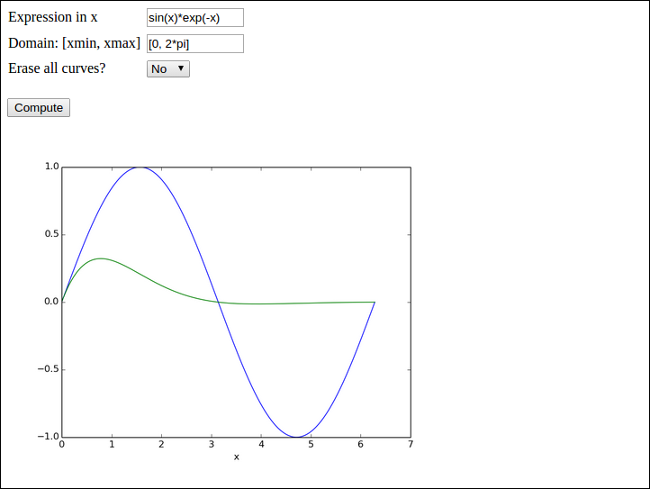
the user has
sin(x)) to be plotted[0, 2*pi])sin(x)*exp(-x))
Hint 1.
You may use the vib1 app from the section Programming the Flask application
with the view_errcheck.html template as starting point.
Preferably, let plots be created as strings, as explained for the vib2
app in the section Avoiding plot files.
The Formula and Domain fields need to be TextField objects,
and the compute function must perform an eval on the user's input.
The Erase field is a SelectField object with selections Yes and
No. The former means that the compute function calls the figure
function in Matplotlib before creating a new plot. If this is not
done, a new formula will be plotting in the same figure as the last one.
With the Yes/No selection, it is possible either plot individual curves
or compare curves in the same plot.
Hint 2.
Performing eval on the user's input requires that names like
sin, exp, and pi are defined. The simplest approach is to
do a
from numpy import *
in the top of the file containing the compute function. All the names
from numpy are then available as global variables and one can simply
do domain = eval(domain) to turn the string domain coming from
the Domain text field into a Python list with two elements.
A better approach is not to rely on global variables, but run eval
in the numpy namespace:
import numpy
domain = eval(domain, numpy.__dict__)
The evaluation of the formula is slightly more complicated if eval
is to be run with the numpy namespace. One first needs
to create \( x \) coordinates:
x = numpy.linspace(domain[0], domain[1], 10001)
Now, eval(formula, numpy.__dict__) will not work because a formula
like sin(x) needs both sin and x in the namespace. The latter
is not in the namespace and must be explicitly included. A new namespace
can be made:
namespace = numpy.__dict__.copy()
namespace.update({'x': x})
formula = eval(formula, namespace)
Hint 3. You should add tests when evaluating and using the strings from input as these may have wrong syntax.
Filename: plot_formula.tar.gz.
This exercise develops a web application that can plot Taylor polynomial approximations of any degree to any user-given formula. You should do Exercise 3: Plot a user-specified formula first as many of the techniques there must be used and even further developed in the present exercise.
The figure below shows an example of what one can do in the web app:
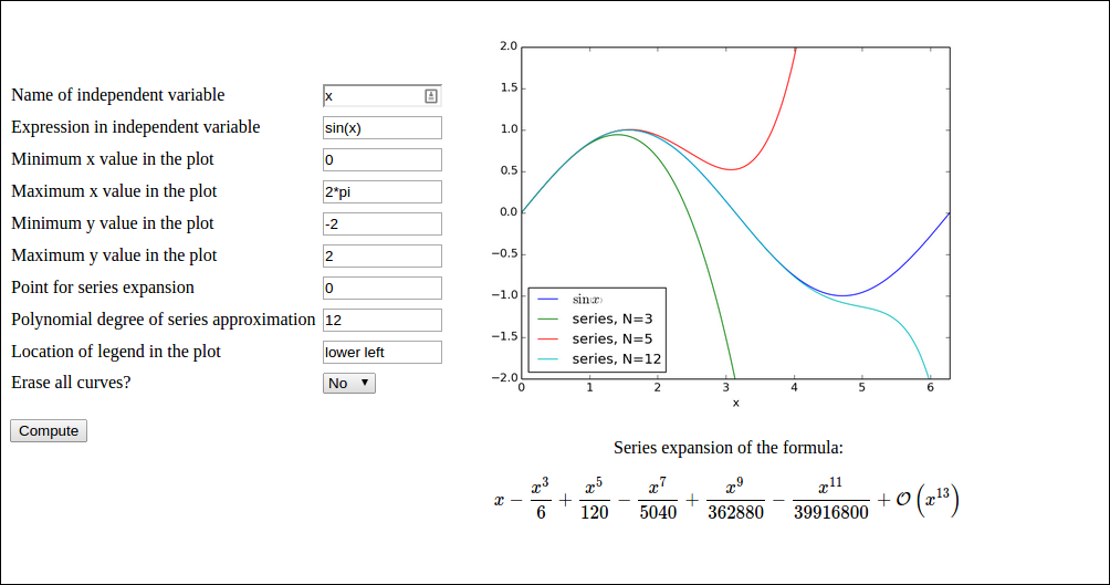
Here, the user has
sin(x))sympy to produce Taylor polynomial expansions of arbitrary
expressions. Here is a session demonstrating how to obtain the
series expansion of \( e^{-x}\sin (\pi x) \) to 2nd degree.
>>> import sympy as sp
>>> x = sp.symbols('x')
>>> f = sp.exp(-x)*sp.sin(sp.pi*x)
>>> f.series(x, 0, 3)
pi*x - pi*x**2 + O(x**3)
>>> sp.latex(f.series(x, 0, 3))
'\\pi x - \\pi x^{2} + \\mathcal{O}\\left(x^{3}\\right)'
>>> fs = f.series(x, 0, 3).removeO()  # get rid of O() term
>>> fs
-pi*x**2 + pi*x
>>> f_func = sp.lambdify([x], fs)     # make Python function
>>> f_func(1)
0.0
>>> f_func(2)
-6.283185307179586
Basically, the steps above must be carried out to create a Python
function for the series expansion such that it can be plotted.
A similar sp.lambdify call on the original formula is also necessary
to plot that one.
However, the challenge is that the formula is available only as a
string, and it may contain an independent variable whose name is also
only available through a string from the web interface. That is, we
may give formulas like exp(-t) if t is chosen as independent
variable. Also, the expression does not contain function names
prefixed with sympy or sp, just plain names like sin, cos,
exp, etc. An example on formula is cos(pi*x) + log(x).
a) Write a function
def formula2series2pyfunc(formula, N, x, x0=0):
that takes a sympy formula, and integer N, a sympy symbol x
and another sympy symbol x0 and returns
1) a Python function for formula, 2) a Python function for the
series expansion of degree N of the formula around x0, and
3) a LaTeX string containing the formula for the series expansion.
Put the function in a file compute.py. You should thereafter be able to run
the following session:
>>> import compute
>>> import sympy as sp
>>> from sympy import *
>>> t = symbols('t')
>>> formula = exp(-2*t)
>>> f, s, latex = compute.formula2series2pyfunc(formula, 3, t)
>>> latex
'- \\frac{4 t^{3}}{3} + 2 t^{2} - 2 t + 1'
>>> import matplotlib.pyplot as plt
>>> import numpy as np
>>> t = np.linspace(0, 2)
>>> plt.plot(t, f(t), t, s(t))
[<matplotlib.lines.Line2D at 0x7fc6c020f350>,
 <matplotlib.lines.Line2D at 0x7fc6c020f5d0>]
>>> plt.show()
The resulting plot is displayed below.
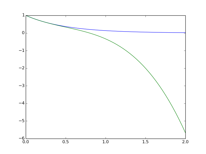
Hint.
The series expansion is obtained by formula.series(x, x0, N),
but the output contains an O() term which makes it impossible to
convert the expression to a Python function via sympy.lambify.
Use
series = formula.series(x, x0, N+1).removeO()
to get an expression that can be used as argument to sympy.lambdify.
We use N+1 since N in the series function refers to the degree
of the O() term, which is now removed.
For the LaTeX expression it is natural to have the O() term:
latex = sympy.latex(formula.series(x, x0, N+1))
because then the terms start with the lowest order (and not the highest
order as is the case when removeO() is used).
b) Write the compute function:
def visualize_series(
    formula,                  # string: formula
    independent_variable,     # string: name of independent var.
    N,                        # int: degree of polynomial approx.
    xmin, xmax, ymin, ymax,   # strings: extent of axes
    legend_loc,               # string: upper left, etc.
    x0='0',                   # string: point of expansion
    erase='yes',              # string: 'yes' or 'no'
    ):
Hint 1.
Converting the string formula to a valid sympy expression is
challenging. First, create a local variable for a sympy symbol
with the content of
independent_variable as name, since such a variable is needed
with performing eval on formula. Also introduce a variable x
to point to the same sympy symbol. Relevant code is
# Turn independent variable into sympy symbol, stored in x
import sympy as sp
exec('x = %s = sp.symbols("%s")' %
     (independent_variable, independent_variable))
Hint 2.
Evaluating formula in the namespace of sympy (so that all the sin,
exp, pi, and similar symbols are defined properly as sympy
objects) needs a merge of the sympy namespace and the variable for
the sympy symbol representing the independent variable:
namespace = sp.__dict__.copy()
local = {}
local[independent_variable] = x
namespace.update(local)
formula = eval(formula, namespace)
Turning x0 into a valid sympy expression is easier: x0 = eval(x0, sp.__dict__).
Hint 3.
Note that in the web interface, the minimum and maximum values on the axis
can be mathematical expressions such as 2*pi. This means that these
quantities must be strings that are evaluated in the numpy namespace, e.g.,
import numpy as np
xmin = eval(xmin, np.__dict__)
Hint 4.
Getting the legends right when plotting multiple curves in the same
plot is a bit tricky. One solution is to have a global variable legends
that is initialized to [] and do the following inside the compute function:
import matplotlib.pyplot as plt
global legends
if erase == 'yes':   # Start new figure?
    plt.figure()
    legends = []
if not legends:
    # We come here every time the figure is empty so
    # we need to draw the formula
    legends.append('$%s$' % sp.latex(formula))
    plt.plot(x, f(x))
Here, f is the Python function for computing the numpy variant
of the expression in formula.
Hint 5.
Use the test block in the file to call the compute function several
times with different values of the erase parameter to test that
the erase functionality is correct.
c) Write the remaining files. These have straightforward content if Exercise 3: Plot a user-specified formula is done and understood.
Filename: Taylor_approx.tar.gz.
gen app
Add a new argument x_axis to the compute function in the
gen
application from the section Autogenerating the code. The x_axis argument measures the extent
of the \( x \) axis in the plots in terms of the number of standard
deviations (default may be 7). Observe how the web interface
automatically adds the new argument and how the plots adapt!
The purpose of this exercise is to look into web apps with multipe submit buttons. More precisely, we want a web app that can perform two actions: add \( a+b \) and multiply \( pq \). There should be two parts of the open web page:
Add button. Clicking on Add
brings up a new line below add: Sum: 3 if \( a+b=3 \).Multiply button. Clicking on Multiply
brings up a new line below add: Product: 5 if \( pq=5 \).
Hint 1.
Make two input form classes, say AddForm and MulForm in model.py.
Since it suffices to fill in either \( a \) and \( b \) or \( p \) and \( q \), all
fields cannot be required.
Let the controller process both classes and collect the two forms
and two results in a form dictionary and a result dictionary
that is passed on the to the view.html file.
Hint 2.
To detect which "subapp" (add or multply) that was used, one can
give a name to the submit button and in the controller check which
of the submit buttons that was pressed (and then perform the associated
computation and update of results). In view.html:
<input type="submit" name="btn" value="Add"></form>
...
<input type="submit" name="btn" value="Multiply"></form>
In controller.py:
if request.method == 'POST' and f.validate() and \
       request.form['btn'] == 'Multiply':
    result['mul'] = mul(f.p.data, f.q.data)
Filename: addmul.tar.gz.
gen app with more data types
In the gen
application from the section Autogenerating the code,
use the label argument in the form field objects to add an
information of the type of data that is to be supplied in the
text field. Extend the model.py file to also handle
lists, tuples, and Numerical Python arrays. For these three
new data types, use a TextField object and run eval
on the text in the view.py file.
A simple test is to extend the compute function with an
argument x_range for the range of the \( x \) axis, specified as
an interval (2-list or 2-tuple).
Filename: gen_ext.tar.gz.
Given a compute with a set of positional and keyword
arguments, the purpose of this exercise is to automatically generate the
Flask files model.py and controller.py. Use the Python inspect
module, see the section Autogenerating the code, to extract
the positional and keyword arguments in compute, and use this
information to construct the relevant Python code in strings. Write
the strings to model.py and controller.py files. Assume as
in the section Autogenerating the code that the user provides
a file view_results.html for defining how the returned object
from the compute function is to be rendered.
Test the code generator on the compute function in the vib1
application to check that the generated
model.py and controller.py files are correct.
Filename: generate_flask.py.
The Bokeh Python library works very well with Flask. The purpose of this exercise is to make a web app where one can explore how parameters in a function influence the function's shape. Given some function \( f(x;p_0,p_1,\ldots,p_n) \), where \( x \) is the independent variable and \( p_0,p_1,\ldots,p_n \) are parameters, we want to create a user interface with a plot field and text fields or sliders for \( p_0,p_1,\ldots,p_n \) such that altering any parameter immediately updates the graph of the \( f \) as a function of \( x \). The Bokeh web side contains a demo: for the specific function $$ f(x;x_0,A,\phi,\omega)= x_0 + A\sin(\omega (x + \phi)).$$ However, this project is about accepting any function \( f(x;p_0,p_1,\ldots,p_n) \) and creating tailored Flask/Bokeh code of the type in the demo. The user must specify a Python function for \( f \):
def f(x, p):
    x_0, A, phi, omega = p
    return x_0 + A*sin(omega*(x - phi))
where p is a list of parameter values. In addition, the user must
provide info about each parameter: the name, a range or a number,
and if range, a default value. Here is an example:
p_info = [
    ('offset', [-2, 2], 0),
    ('amplitude', [0, 5], 2.5),
    ('phase', 0),
    ('frequency', [1, 10], 1)]
Parameters with an interval range get a slider for setting the value,
while parameters with only a number, as for phase in this example,
get a text field where the user can alter the number.
The user must also provide a suitable range for the \( x \) axis. As test case beyond the example above, try a Gaussian function with this input from the user:
import numpy as np

def gaussian(x, p):
    mu, sigma = p
    return 1./(sigma*np.sqrt(2*np.pi))*\
           np.exp(-0.5*(x - mu)**2/sigma**2)

p_info = [
    ('mean', [-2, 2], 0),
    ('standard deviation', [0.1, 4], 1)]

x_axis = [-10, 10]
Filename: expore_func.tar.gz.
numpy, scipy, or matplotlib)