Exercises

Exercise 1: Add two numbers

Make a web application that reads two numbers from a web page, adds the numbers, and prints the sum in a new web page. Package the necessary files that constitute the application in a tar file. Filename: add2.tar.gz.

Exercise 2: Upload data file and visualize curves

Suppose you have tabular data in a file:

#  t        y       error
0.0000    1.2345   1.4E-4
1.0000    0.9871  -4.9E-3
1.2300    0.5545   8.2E-3

That is, there is a comment line with headings for the various columns, and then floating-point values are listed with an arbitrary number of columns and rows. You want to upload such a data file to a web application and have the each column, from the second one, plotted against the the values in the first column. In the particular example, y and error should be plotted against t, yielding two curves.

The web application may have one field: the name of the file to upload. Search for constructions on how to upload a files and write this application. Generate a suitable data file for testing purposes. Filename: upload.tar.gz.

Exercise 3: Plot a user-specified formula

The purpose of this exercise is to write a web application that can visualize any user-given formula. For example, in the interface below,

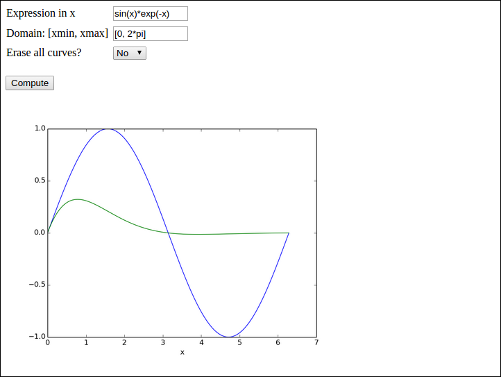
the user has

specified a curve \( \sin (x) \) (sin(x)) to be plotted
specified the \( x \) interval to be \( [0,2\pi] \) ([0, 2*pi])
clicked Compute to get a blue line with the sine curve
specified a new formula \( \sin(x)e^{-x} \) (sin(x)*exp(-x))
chosen No as the answer to Erase all curves?
clicked Compute to have the \( \sin(x)e^{-x} \) drawn with green line without erasing the previous curve

That is, the user can fill in any expression in \( x \), specify the domain for plotting, and choose whether new curves should be added to the plot or if all curves should be erased prior to drawing a new one.

Hint 1.

Performing eval on the user's input requires that names like sin, exp, and pi are defined. The simplest approach is to do a

from numpy import *

in the top of the file containing the compute function. All the names from numpy are then available as global variables and one can simply do domain = eval(domain) to turn the string domain coming from the Domain text field into a Python list with two elements.

A better approach is not to rely on global variables, but run eval in the numpy namespace:

import numpy
domain = eval(domain, numpy.__dict__)

The evaluation of the formula is slightly more complicated if eval is to be run with the numpy namespace. One first needs to create \( x \) coordinates:

x = numpy.linspace(domain[0], domain[1], 10001)

Now, eval(formula, numpy.__dict__) will not work because a formula like sin(x) needs both sin and x in the namespace. The latter is not in the namespace and must be explicitly included. A new namespace can be made:

namespace = numpy.__dict__.copy()
namespace.update({'x': x})
formula = eval(formula, namespace)

Hint 2.

You should add tests when evaluating and using the strings from input as these may have wrong syntax.

Filename: plot_formula.tar.gz.

Exercise 4: Visualize Taylor polynomial approximations

This exercise develops a web application that can plot Taylor polynomial approximations of any degree to any user-given formula. You should do Exercise 3: Plot a user-specified formula first as many of the techniques there must be used and even further developed in the present exercise.

The figure below shows an example of what one can do in the web app:

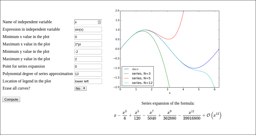
Here, the user has

filled in the formula \( \sin(x) \) (sin(x))
specified N to be 3
clicked Compute to get the formula \( \sin(x) \) plotted together with the Taylor polynomial approximation of degree 3, expanded around \( x=0 \)
changed N to 5
chosen No for the question Erase all curves?
clicked Compute to have the series expansion of degree 5 plotted in the same plot
changed N to 10
clicked Compute to have the series expansion of degree 10 plotted in the same plot

We can use sympy to produce Taylor polynomial expansions of arbitrary expressions. Here is a session demonstrating how to obtain the series expansion of \( e^{-x}\sin (\pi x) \) to 2nd degree.

>>> import sympy as sp
>>> x = sp.symbols('x')
>>> f = sp.exp(-x)*sp.sin(sp.pi*x)
>>> f.series(x, 0, 3)
pi*x - pi*x**2 + O(x**3)
>>> sp.latex(f.series(x, 0, 3))
'\\pi x - \\pi x^{2} + \\mathcal{O}\\left(x^{3}\\right)'
>>> fs = f.series(x, 0, 3).removeO()  # get rid of O() term
>>> fs
-pi*x**2 + pi*x
>>> f_func = sp.lambdify([x], fs)     # make Python function
>>> f_func(1)
0.0
>>> f_func(2)
-6.283185307179586

Basically, the steps above must be carried out to create a Python function for the series expansion such that it can be plotted. A similar sp.lambdify call on the original formula is also necessary to plot that one.

However, the challenge is that the formula is available only as a string, and it may contain an independent variable whose name is also only available through a string from the web interface. That is, we may give formulas like exp(-t) if t is chosen as independent variable. Also, the expression does not contain function names prefixed with sympy or sp, just plain names like sin, cos, exp, etc. An example on formula is cos(pi*x) + log(x).

a) Write a function

def formula2series2pyfunc(formula, N, x, x0=0):

that takes a sympy formula, and integer N, a sympy symbol x and another sympy symbol x0 and returns 1) a Python function for formula, 2) a Python function for the series expansion of degree N of the formula around x0, and 3) a LaTeX string containing the formula for the series expansion.

Put the function in a file compute.py. You should thereafter be able to run the following session:

>>> import compute
>>> import sympy as sp
>>> from sympy import *
>>> t = symbols('t')
>>> formula = exp(-2*t)
>>> f, s, latex = compute.formula2series2pyfunc(formula, 3, t)
>>> latex
'- \\frac{4 t^{3}}{3} + 2 t^{2} - 2 t + 1'
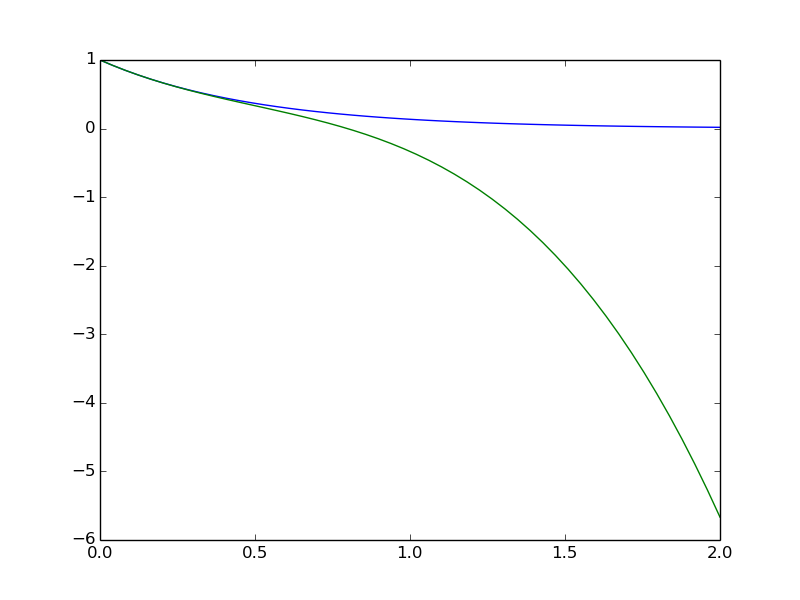
>>> import matplotlib.pyplot as plt
>>> import numpy as np
>>> t = np.linspace(0, 2)
>>> plt.plot(t, f(t), t, s(t))
[<matplotlib.lines.Line2D at 0x7fc6c020f350>,
 <matplotlib.lines.Line2D at 0x7fc6c020f5d0>]
>>> plt.show()

The resulting plot is displayed below.

Hint.

The series expansion is obtained by formula.series(x, x0, N), but the output contains an O() term which makes it impossible to convert the expression to a Python function via sympy.lambify. Use

series = formula.series(x, x0, N+1).removeO()

to get an expression that can be used as argument to sympy.lambdify. We use N+1 since N in the series function refers to the degree of the O() term, which is now removed.

For the LaTeX expression it is natural to have the O() term:

latex = sympy.latex(formula.series(x, x0, N+1))

because then the terms start with the lowest order (and not the highest order as is the case when removeO() is used).

b) Write the compute function:

def visualize_series(
    formula,                  # string: formula
    independent_variable,     # string: name of independent var.
    N,                        # int: degree of polynomial approx.
    xmin, xmax, ymin, ymax,   # strings: extent of axes
    legend_loc,               # string: upper left, etc.
    x0='0',                   # string: point of expansion
    erase='yes',              # string: 'yes' or 'no'
    ):

Hint 1.

Converting the string formula to a valid sympy expression is challenging. First, create a local variable for a sympy symbol with the content of independent_variable as name, since such a variable is needed with performing eval on formula. Also introduce a variable x to point to the same sympy symbol. Relevant code is

# Turn independent variable into sympy symbol, stored in x
import sympy as sp
exec('x = %s = sp.symbols("%s")' %
     (independent_variable, independent_variable))

Hint 2.

Evaluating formula in the namespace of sympy (so that all the sin, exp, pi, and similar symbols are defined properly as sympy objects) needs a merge of the sympy namespace and the variable for the sympy symbol representing the independent variable:

namespace = sp.__dict__.copy()
local = {}
local[independent_variable] = x
namespace.update(local)
formula = eval(formula, namespace)

Turning x0 into a valid sympy expression is easier: x0 = eval(x0, sp.__dict__).

Hint 3.

Note that in the web interface, the minimum and maximum values on the axis can be mathematical expressions such as 2*pi. This means that these quantities must be strings that are evaluated in the numpy namespace, e.g.,

import numpy as np
xmin = eval(xmin, np.__dict__)

Hint 4.

Getting the legends right when plotting multiple curves in the same plot is a bit tricky. One solution is to have a global variable legends that is initialized to [] and do the following inside the compute function:

import matplotlib.pyplot as plt
global legends
if erase == 'yes':   # Start new figure?
    plt.figure()
    legends = []
if not legends:
    # We come here every time the figure is empty so
    # we need to draw the formula
    legends.append('$%s$' % sp.latex(formula))
    plt.plot(x, f(x))

Here, f is the Python function for computing the numpy variant of the expression in formula.

Hint 5.

Use the test block in the file to call the compute function several times with different values of the erase parameter to test that the erase functionality is correct.

c) Write the remaining files. These have straightforward content if Exercise 3: Plot a user-specified formula is done and understood.

Filename: Taylor_approx.tar.gz.

Django4scientists

Exercises

Exercise 1: Add two numbers

Exercise 2: Upload data file and visualize curves

Exercise 3: Plot a user-specified formula

Exercise 4: Visualize Taylor polynomial approximations

Django resources