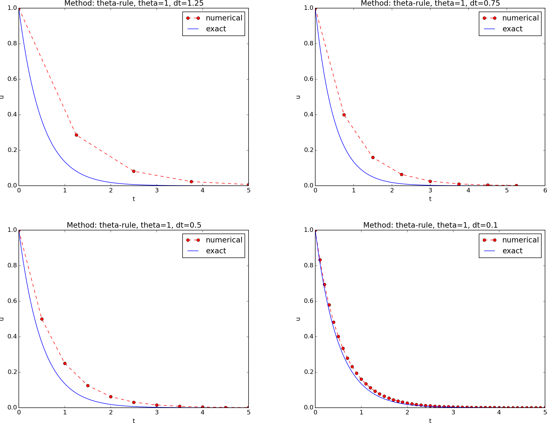
Figure 1: The Backward Euler method for decreasing time step values.
Summary. This report investigates the accuracy of three finite difference schemes for the ordinary differential equation \( u'=-au \) with the aid of numerical experiments. Numerical artifacts are in particular demonstrated.
Mathematical problem
Numerical solution method
Implementation
Numerical experiments
Error vs \( \Delta t \)
Bibliography
We address the initial-value problem $$ \begin{align} u'(t) &= -au(t), \quad t \in (0,T], \label{ode}\\ u(0) &= I, \label{initial:value} \end{align} $$ where \( a \), \( I \), and \( T \) are prescribed parameters, and \( u(t) \) is the unknown function to be estimated. This mathematical model is relevant for physical phenomena featuring exponential decay in time, e.g., vertical pressure variation in the atmosphere, cooling of an object, and radioactive decay.
We introduce a mesh in time with points \( 0 = t_0 < t_1 \cdots < t_{N_t}=T \). For simplicity, we assume constant spacing \( \Delta t \) between the mesh points: \( \Delta t = t_{n}-t_{n-1} \), \( n=1,\ldots,N_t \). Let \( u^n \) be the numerical approximation to the exact solution at \( t_n \).
The \( \theta \)-rule [1] is used to solve \eqref{ode} numerically: $$ u^{n+1} = \frac{1 - (1-\theta) a\Delta t}{1 + \theta a\Delta t}u^n, $$ for \( n=0,1,\ldots,N_t-1 \). This scheme corresponds to
The numerical method is implemented in a Python function
[2] solver (found in the model.py Python module file):
def solver(I, a, T, dt, theta):
    """Solve u'=-a*u, u(0)=I, for t in (0,T] with steps of dt."""
    dt = float(dt)            # avoid integer division
    Nt = int(round(T/dt))     # no of time intervals
    T = Nt*dt                 # adjust T to fit time step dt
    u = zeros(Nt+1)           # array of u[n] values
    t = linspace(0, T, Nt+1)  # time mesh

    u[0] = I                  # assign initial condition
    for n in range(0, Nt):    # n=0,1,...,Nt-1
        u[n+1] = (1 - (1-theta)*a*dt)/(1 + theta*dt*a)*u[n]
    return u, t
A set of numerical experiments has been carried out, where \( I \), \( a \), and \( T \) are fixed, while \( \Delta t \) and \( \theta \) are varied. In particular, \( I=1 \), \( a=2 \), \( \Delta t = 1.25, 0.75, 0.5, 0.1 \). Figure 1 contains four plots, corresponding to four decreasing \( \Delta t \) values. The red dashed line represent the numerical solution computed by the Backward Euler scheme, while the blue line is the exact solution. The corresponding results for the Crank-Nicolson and Forward Euler methods appear in Figures 2 and 3.
Figure 1: The Backward Euler method for decreasing time step values.
Figure 2: The Crank-Nicolson method for decreasing time step values.
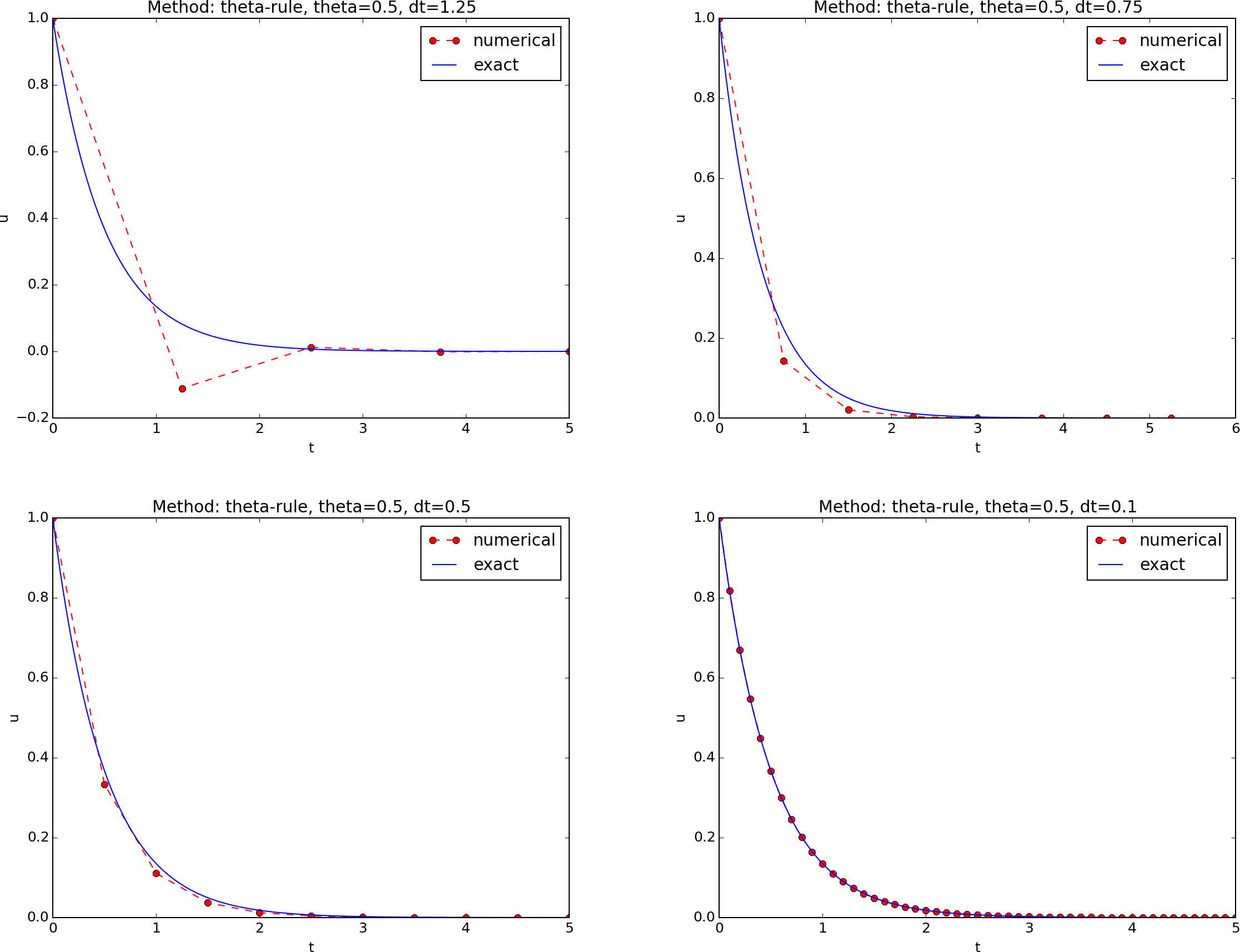
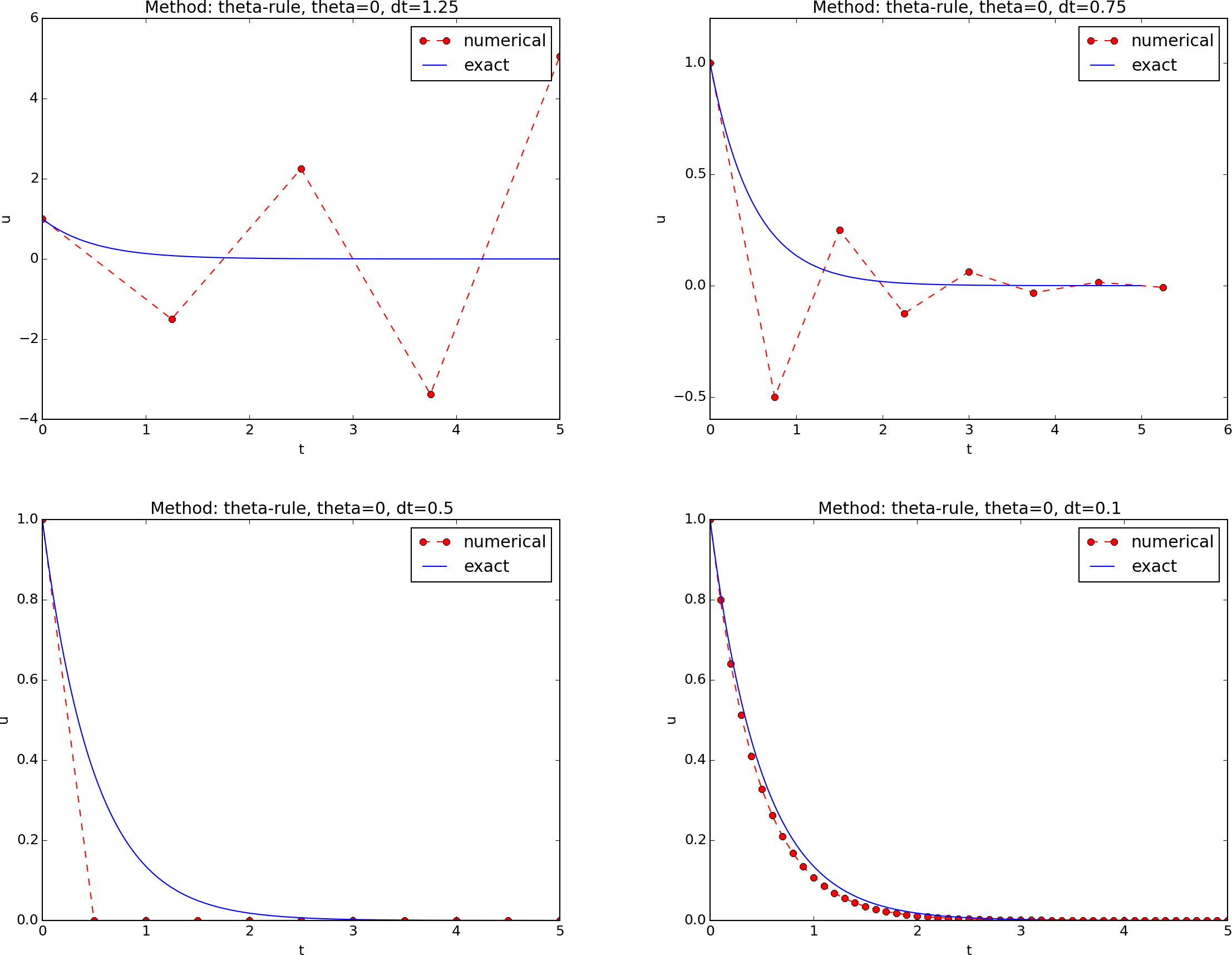
Figure 3: The Forward Euler method for decreasing time step values.
How the error $$ E^n = \left(\int_0^T (Ie^{-at} - u^n)^2dt\right)^{\frac{1}{2}}$$ varies with \( \Delta t \) for the three numerical methods is shown in Figure 4.
The data points for the three largest \( \Delta t \) values in the Forward Euler method are not relevant as the solution behaves non-physically.
Figure 4: Variation of the error with the time step.
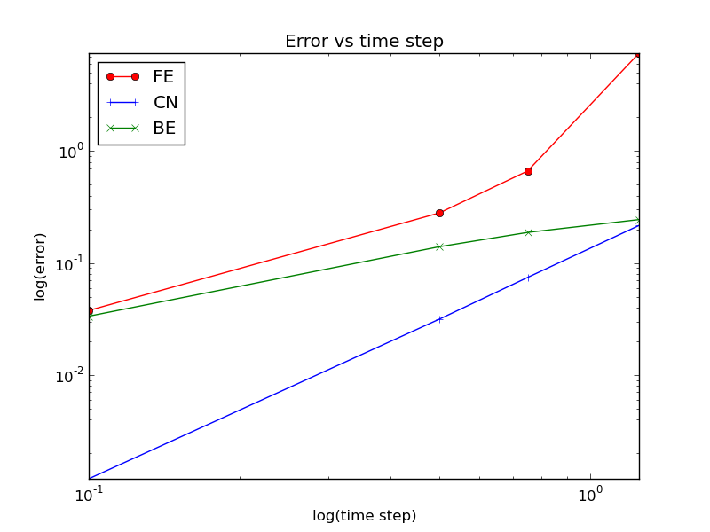
The \( E \) numbers corresponding to Figure 4 are given in the table below.
| \( \Delta t \) | \( \theta=0 \) | \( \theta=0.5 \) | \( \theta=1 \) |
| 1.25 | 7.4630 | 0.2161 | 0.2440 |
| 0.75 | 0.6632 | 0.0744 | 0.1875 |
| 0.50 | 0.2797 | 0.0315 | 0.1397 |
| 0.10 | 0.0377 | 0.0012 | 0.0335 |