Monte Carlo Simulation with Cython

Author:Hans Petter Langtangen Date:Sep 24, 2012

Monte Carlo simulations are usually known to require long execution times. Implementing such simulations in pure Python may lead to inefficient code. The purpose of this note is to show how Python implementations of Monte Carlo simulations, can be made much more efficient by porting the code to Cython. Pure C implementations are included for comparison of efficiency. The reader should know about basic Python and perhaps a bit about Monte Carlo simulations. Cython will be introduced in a step-by-step fashion

Pure Python Code for Monte Carlo Simulation

A short, intuitive algorithm in Python is first developed. Then this code is vectorized using functionality of the Numerical Python package. Later sections migrate the algorithm to Cython code and also plain C code for comparison. At the end the various techniques are ranked according to their computational efficiency.

The Computational Problem

A die is thrown \(m\) times. What is the probability of getting six eyes at least \(n\) times? For example, if \(m=5\) and \(n=3\), this is the same as asking for the probability that three or more out of five dice show six eyes.

The probability can be estimated by Monte Carlo simulation. We simulate the process a large number of times, \(N\), and count how many times, \(M\), the experiment turned out successfully, i.e., when we got at least \(n\) out of \(m\) dice with six eyes in a throw.

Monte Carlo simulation has traditionally been viewed as a very costly computational method, normally requiring very sophisticated, fast computer implementations in compiled languages. An interesting question is how useful high-level languages like Python and associated tools are for Monte Carlo simulation. This will now be explored.

A Scalar Python Implementation

Let us introduce the more descriptive variables ndice for \(m\) and nsix for \(n\). The Monte Carlo method is simply a loop, repeated N times, where the body of the loop may directly express the problem at hand. Here, we draw ndice random integers r in \([1,6]\) inside the loop and count of many (six) that equal 6. If six >= nsix, the experiment is a success and we increase the counter M by one.

A Python function implementing this approach may look as follows:

import random

def dice6_py(N, ndice, nsix):
    M = 0                     # no of successful events
    for i in range(N):        # repeat N experiments
        six = 0               # how many dice with six eyes?
        for j in range(ndice):
            r = random.randint(1, 6)  # roll die no. j
            if r == 6:
               six += 1
        if six >= nsix:       # successful event?
            M += 1
    p = float(M)/N
    return p

The float(M) transformation is important since M/N will imply integer division when M and N both are integers in Python v2.x and many other languages.

We will refer to this implementation is the plain Python implementation. Timing the function can be done by:

import time
t0 = time.clock()
p = dice6_py(N, ndice, nsix)
t1 = time.clock()
print 'CPU time for loops in Python:', t1-t0

The table to appear later shows the performance of this plain, pure Python code relative to other approaches. There is a factor of 30+ to be gained in computational efficiency by reading on.

The function above can be verified by studying the (somewhat simplified) case \(m=n\) where the probability becomes \(6^{-n}\). The probability quickly becomes small with increasing \(n\). For such small probabilities the number of successful events \(M\) is small, and \(M/N\) will not be a good approximation to the probability unless \(M\) is reasonably large, which requires a very large \(N\). For example, with \(n=4\) and \(N=10^5\) the average probability in 25 full Monte Carlo experiments is 0.00078 while the exact answer is 0.00077. With \(N=10^6\) we get the two correct significant digits from the Monte Carlo simulation, but the extra digit costs a factor of 10 in computing resources since the CPU time scales linearly with \(N\).

A Vectorized Python Implementation

A vectorized version of the previous program consists of replacing the explicit loops in Python by efficient operations on vectors or arrays, using functionality in the Numerical Python (numpy) package. Each array operation takes place in C or Fortran and is hence much more efficient than the corresponding loop version in Python.

First, we must generate all the random numbers to be used in one operation, which runs fast since all numbers are then calculated in efficient C code. This is accomplished using the numpy.random module. Second, the analysis of the large collection of random numbers must be done by appropriate vector/array operations such that no looping in Python is needed. The solution algorithm must therefore be expressed through a series of function calls to the numpy library. Vectorization requires knowledge of the library’s functionality and how to assemble the relevant building blocks to an algorithm without operations on individual array elements.

Generation of ndice random number of eyes for N experiments is performed by

import numpy as np
eyes = np.random.random_integers(1, 6, size=(N, ndice))

Each row in the eyes array corresponds to one Monte Carlo experiment.

The next step is to count the number of successes in each experiment. This counting should not make use of any loop. Instead we can test eyes == 6 to get a boolean array where an element i,j is True if throw (or die) number j in Monte Carlo experiment number i gave six eyes. Summing up the rows in this boolean array (True is interpreted as 1 and False as 0), we are interested in the rows where the sum is equal to or greater than nsix, because the number of such rows equals the number of successful events. The vectorized algorithm can be expressed as

def dice6_vec1(N, ndice, nsix):
    eyes = np.random.random_integers(1, 6, size=(N, ndice))
    compare = eyes == 6
    throws_with_6 = np.sum(compare, axis=1)  # sum over columns
    nsuccesses = throws_with_6 >= nsix
    M = np.sum(nsuccesses)
    p = float(M)/N
    return p

The use of np.sum instead of Python’s own sum function is essential for the speed of this function: using M = sum(nsucccesses) instead slows down the code by a factor of almost 10! We shall refer to the dice6_vec1 function as the vectorized Python, version1 implementation.

The criticism against the vectorized version is that the original problem description, which was almost literally turned into Python code in the dice6_py function, has now become much more complicated. We have to decode the calls to various numpy functionality to actually realize that dice6_py and dice6_vec correspond to the same mathematics.

Here is another possible vectorized algorithm, which is easier to understand, because we retain the Monte Carlo loop and vectorize only each individual experiment:

def dice6_vec2(N, ndice, nsix):
    eyes = np.random.random_integers(1, 6, (N, ndice))
    six = [6 for i in range(ndice)]
    M = 0
    for i in range(N):
        # Check experiment no. i:
        compare = eyes[i,:] == six
        if np.sum(compare) >= nsix:
            M += 1
    p = float(M)/N
    return p

We refer to this implementation as vectorized Python, version 2. As will be shown later, this implementation is significantly slower than the plain Python implementation (!) and very much slower than the vectorized Python, version 1 approach. A conclusion is that readable, partially vectorized code, may run slower than straightforward scalar code.

Migrating Scalar Python Code to Cython

A Plain Cython Implementation

A Cython program starts with the scalar Python implementation, but all variables are specified with their types, using Cython’s variable declaration syntax, like cdef int M = 0 where we in standard Python just write M = 0. Adding such variable declarations in the scalar Python implementation is straightforward:

import random

def dice6_cy1(int N, int ndice, int nsix):
    cdef int M = 0            # no of successful events
    cdef int six, r
    cdef double p
    for i in range(N):        # repeat N experiments
        six = 0               # how many dice with six eyes?
        for j in range(ndice):
            r = random.randint(1, 6)  # roll die no. j
            if r == 6:
               six += 1
        if six >= nsix:       # successful event?
            M += 1
    p = float(M)/N
    return p

This code must be put in a separate file with extension .pyx. Running Cython on this file translates the Cython code to C. Thereafter, the C code must be compiled and linked to form a shared library, which can be imported in Python as a module. All these tasks are normally automated by a setup.py script. Let the dice6_cy1 function above be stored in a file dice6.pyx. A proper setup.py script looks as follows:

from distutils.core import setup
from distutils.extension import Extension
from Cython.Distutils import build_ext

setup(
  name='Monte Carlo simulation',
  ext_modules=[Extension('_dice6_cy', ['dice6.pyx'],)],
  cmdclass={'build_ext': build_ext},
)

Running

Terminal> python setup.py build_ext --inplace

generates the C code and creates a (shared library) file _dice6_cy.so (known as a C extension module) which can be loaded into Python as a module with name _dice6_cy:

from _dice6_cy import dice6_cy1
import time
t0 = time.clock()
p = dice6_cy1(N, ndice, nsix)
t1 = time.clock()
print t1 - t0

We refer to this implementation as Cython random.randint. Although most of the statements in the dice6_cy1 function are turned into plain and fast C code, the speed is not much improved compared with the original scalar Python code.

To investigate what takes time in this Cython implementation, we can perform a profiling. The template for profiling a Python function whose call syntax is stored in some string statement, reads

import cProfile, pstats
cProfile.runctx(statement, globals(), locals(), '.prof')
s = pstats.Stats('.prof')
s.strip_dirs().sort_stats('time').print_stats(30)

Here, we set

statement = 'dice6_cy1(N, ndice, nsix)'

In addition, a Cython file in which there are functions we want to profile must start with the line

# cython: profile=True

to turn on profiling when creating the extension module. The profiling output from the present example looks like

       5400004 function calls in 7.525 CPU seconds

 Ordered by: internal time

 ncalls  tottime  percall  cumtime  percall filename:lineno(function)
1800000    4.511    0.000    4.863    0.000 random.py:160(randrange)
1800000    1.525    0.000    6.388    0.000 random.py:224(randint)
      1    1.137    1.137    7.525    7.525 dice6.pyx:6(dice6_cy1)
1800000    0.352    0.000    0.352    0.000 {method 'random' ...
      1    0.000    0.000    7.525    7.525 {dice6_cy.dice6_cy1}

We easily see that it is the call to random.randint that consumes almost all the time. The reason is that the generated C code must call a Python module (random), which implies a lot of overhead. The C code should only call plain C functions, or if Python functions must be called, they should involve so much computations that the overhead in calling Python from C is negligible.

Instead of profiling the code to uncover inefficient constructs we can generate a visual representation of how the Python code is translated to C. Running

Terminal> cython -a dice6.pyx

creates a file dice6.html which can be loaded into a web browser to inspect what Cython has done with the Python code.

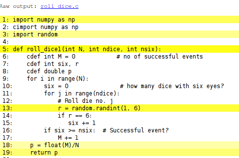
White lines indicate that the Python code is translated into C code, while the yellow lines indicate that the generated C code must make calls back to Python (using the Python C API, which implies overhead). Here, the random.randint call is in yellow, so this call is not translated to efficient C code.

A Better Cython Implementation

To speed up the previous Cython code, we have to get rid of the random.randint call every time we need a random variable. Either we must call some C function for generating a random variable or we must create a bunch of random numbers simultaneously as we did in the vectorized functions shown above. We first try the latter well-known strategy and apply the numpy.random module to generate all the random numbers we need at once:

import  numpy as np
cimport numpy as np

cdef np.ndarray[np.int_t,
                ndim=2,
                negative_indices=False,
                mode='c'] eyes = \
                np.random.random_integers(1, 6, (N, ndice))

This code needs some explanation. The cimport statement imports a special version of numpy for Cython and is needed after the standard numpy import. The declaration of the array of random numbers could just go as

cdef np.ndarray eyes = np.random.random_integers(1, 6, (N, ndice))

However, the processing of the eyes array will then be slow because Cython does not have enough information about the array. To generate optimal C code, we must provide information on the element types in the array, the number of dimensions of the array, that the array is stored in contiguous memory, and that we do not need negative indices (which slows down array indexing). All this information is inserted in square brackets: np.int_t denotes integer array elements (np.int is the usual data type object, but np.int_t is a Cython precompiled version of this object), ndim=2 tells that the array has two dimensions (indices), negative_indices=False turns off the possibility for negative indices (counting from the end), and mode='c' indicates contiguous storage of the array. We also insert a line @cython.boundscheck(False) at the line before the function to tell Cython to turn off the costly check that array indices stay within their bounds. With all this extra information, Cython can generate C code that works with numpy arrays as efficiently as native C arrays.

The rest of the code is a plain copy of the dice6_py function, but with the random.randint call replaced by an array look-up eyes[i,j] to retrieve the next random number. The two loops will now be as efficient as if they were coded directly in pure C.

The complete code for the efficient version of the dice6_cy1 function looks as follows:

import  numpy as np
cimport numpy as np
import cython
@cython.boundscheck(False)
def dice6_cy2(int N, int ndice, int nsix):
    # Use numpy to generate all random numbers
    cdef int M = 0            # no of successful events
    cdef int six, r
    cdef double p
    cdef np.ndarray[np.int_t,
                    ndim=2,
                    negative_indices=False,
                    mode='c'] eyes = \
                    np.random.random_integers(1, 6, (N, ndice))
    for i in range(N):
        six = 0               # how many dice with six eyes?
        for j in range(ndice):
            r = eyes[i,j]     # roll die no. j
            if r == 6:
               six += 1
        if six >= nsix:       # successful event?
            M += 1
    p = float(M)/N
    return p

This Cython implementation is named Cython numpy.random.

The disadvantage with the dice6_cy2 function is that large simulations (large N) also require large amounts of memory, which usually limits the possibility for high accuracy much more than the CPU time. It would be advantageous to have a fast random number generator a la random.randint in C. The C library stdlib has a generator of random integers, rand(), generating numbers from 0 to up RAND_MAX. Both the rand function and the RAND_MAX integer are easy to access in a Cython program:

from libc.stdlib cimport rand, RAND_MAX

r = 1 + int(rand()/(RAND_MAX*6.0)) # random integer 1,...,6

Note that rand() returns an integer so we must avoid integer division by ensuring that the denominator is a real number. We also need to explicitly convert the resulting real fraction to int since r is declared as int.

With this way of generating random numbers we can create a version of dice6_cy1 that is as fast as dice6_cy, but avoids all the memory demands and the somewhat complicated array declarations of the latter:

from libc.stdlib cimport rand, RAND_MAX
def dice6_cy3(int N, int ndice, int nsix):
    cdef int M = 0            # no of successful events
    cdef int six, r
    cdef double p
    for i in range(N):
        six = 0               # how many dice with six eyes?
        for j in range(ndice):
            # Roll die no. j
            r = 1 + int(rand()/(RAND_MAX*6.0))
            if r == 6:
               six += 1
        if six >= nsix:       # successful event?
            M += 1
    p = float(M)/N
    return p

This final Cython implementation will be referred to as Cython stdlib.rand.

Migrating Code to C

Writing a C Program

A natural next improvement would be to program the Monte Carlo simulation loops directly in a compiled programming language, which guarantees optimal speed. Here we choose the C programming language for this purpose. The C version of our dice6 function and an associated main program take the form

#include <stdio.h>
#include <stdlib.h>

double dice6(int N, int ndice, int nsix)
{
  int M = 0;
  int six, r, i, j;
  double p;

  for (i = 0; i < N; i++) {
    six = 0;
    for (j = 0; j < ndice; j++) {
      r = 1 + rand()/(RAND_MAX*6.0); /* roll die no. j */
      if (r == 6)
        six += 1;
    }
    if (six >= nsix)
      M += 1;
  }
  p = ((double) M)/N;
  return p;
}

int main(int nargs, const char* argv[])
{
  int N = atoi(argv[1]);
  int ndice = 6;
  int nsix = 3;
  double p = dice6(N, ndice, nsix);
  printf("C code: N=%d, p=%.6f\n", N, p);
  return 0;
}

This code is placed in a file dice6_c.c. The file can typically be compiled and run by

Terminal> gcc -O3 -o dice6.capp dice6_c.c
Terminal> ./dice6.capp 1000000

This solution is later referred to as C program.

Migrating Loops to C Code via F2PY

Instead of programming the whole application in C, we may consider migrating the loops to the C function dice6 shown above and then have the rest of the program (essentially the calling main program) in Python. This is a convenient solution if we were to do many other, less CPU-time critical things for convenience in Python.

There are many alternative techniques for calling C functions from Python. Here we shall explain two. The first applies the program f2py to generate the necessary code that glues Python and C. The f2py program was actually made for gluing Python and Fortran, but it can work with C too. We need a specification of the C function to call in terms of a Fortran 90 module. Such a module can be written by hand, but f2py can also generate it. To this end, we make a Fortran file dice6_c_signature.f with the signature of the C function written in Fortran 77 syntax with some annotations:

real*8 function dice6(n, ndice, nsix)
Cf2py intent(c) dice6
      integer n, ndice, nsix
Cf2py intent(c) n, ndice, nsix
      return
      end

The annotations intent(c) are necessary to tell f2py that the Fortran variables are to be treated as plain C variables and not as pointers (which is the default interpretation of variables in Fortran). The C2fpy are special comment lines that f2py recognizes, and these lines are used to provide extra information to f2py which have no meaning in plain Fortran 77.

We must run f2py to generate a .pyf file with a Fortran 90 module specification of the C function to call:

Terminal> f2py -m _dice6_c1 -h dice6_c.pyf \
          dice6_c_signature.f

Here _dice6_c1 is the name of the module with the C function that is to be imported in Python, and dice6_c.pyf is the name of the Fortran 90 module file to be generated. Programmers who know Fortran 90 may want to write the dice6_c.pyf file by hand.

The next step is to use the information in dice6_c.pyf to generate a (C extension) module _dice6_c1. Fortunately, f2py generates the necessary code, and compiles and links the relevant files, to form a shared library file _dice6_c1.so, by a short command:

Terminal> f2py -c dice6_c.pyf dice6_c.c

We can now test the module:

>>> import _dice6_c1
>>> print dir(_dice6_c1)  # module contents
['__doc__', '__file__', '__name__', '__package__',
 '__version__', 'dice6']
>>> print _dice6_c1.dice6.__doc__
dice6 - Function signature:
  dice6 = dice6(n,ndice,nsix)
Required arguments:
  n : input int
  ndice : input int
  nsix : input int
Return objects:
  dice6 : float
>>> _dice6_c1.dice6(N=1000, ndice=4, nsix=2)
0.145

The method of calling the C function dice6 via an f2py generated module is referred to as C via f2py.

Migrating Loops to C Code via Cython

The Cython tool can also be used to call C code, not only generating C code from the Cython language. Our C code is in the file dice6_c.c, but for Cython to see this code we need to create a header file dice6_c.h listing the definition of the function(s) we want to call from Python. The header file takes the form

#include <stdio.h>
#include <stdlib.h>

extern double dice6(int N, int ndice, int nsix);

The next step is to make a .pyx file with a definition of the C function from the header file and a Python function that calls the C function:

cdef extern from "dice6_c.h":
    double dice6(int N, int ndice, int nsix)

def dice6_cwrap(int N, int ndice, int nsix):
    return dice6(N, ndice, nsix)

Cython must use this file, named dice6_cwrap.pyx, to generate C code, which is to be compiled and linked with the dice6_c.c code. All this is accomplished in a setup.py script:

from distutils.core import setup
from distutils.extension import Extension
from Cython.Distutils import build_ext

sources = ['dice6_cwrap.pyx', 'dice6_c.c']

setup(
  name='Monte Carlo simulation',
  ext_modules=[Extension('_dice6_c2', sources)],
  cmdclass={'build_ext': build_ext},
)

This setup.py script is run as

Terminal> python setup.py build_ext --inplace

resulting in a shared library file _dice6_c2.so, which can be loaded into Python as a module:

>>> import _dice6_c2
>>> print dir(_dice6_c2)
['__builtins__', '__doc__', '__file__', '__name__',
 '__package__', '__test__', 'dice6_cwrap']

We see that the module contains the function dice6_cwrap, which was made to call the underlying C function dice6.

Comparing Efficiency

All the files corresponding to the various techniques described above are available as a tarball or accessible from through the GitHub project MC_cython. A file make.sh performs all the compilations, while compare.py runs all methods and prints out the CPU time required by each method, normalized by the fastest approach. The results for \(N=450,000\) are listed below (MacBook Air running Ubuntu in a VMWare Fusion virtual machine).

Method	Timing
C program	1.0
Cython stdlib.rand	1.2
Cython numpy.random	1.2
C via f2py	1.2
C via Cython	1.2
vectorized Python, version 1	1.9
Cython random.randint	33.6
plain Python	37.7
vectorized Python, version 2	105.0

The CPU time of the plain Python version was 10 s, which is reasonably fast for obtaining a fairly accurate result in this problem. The lesson learned is therefore that a Monte Carlo simulation can be implemented in plain Python first. If more speed is needed, one can just add type information and create a Cython code. Studying the HTML file with what Cython manages to translate to C may give hints about how successful the Cython code is and point to optimizations, like avoiding the call to random.randint in the present case. Optimal Cython code runs here at approximately the same speed as calling a handwritten C function with the time-consuming loops. It is to be noticed that the stand-alone C program here ran faster than calling C from Python, probably because the amount of calculations is not large enough to make the overhead of calling C negligible.

Vectorized Python do give a great speed-up compared to plain loops in Python, if done correctly, but the efficiency is not on par with Cython or handwritten C. Even more important is the fact that vectorized code is not at all as readable as the algorithm expressed in plain Python, Cython, or C. Cython therefore provides a very attractive combination of readability, ease of programming, and high speed.