Ch.8: Random numbers and simple games
Aug 15, 2015
Use of random numbers in programs
|
|
|
Random numbers are used to simulate uncertain events
- Some problems in science and technology are desrcribed by "exact" mathematics, leading to "precise" results
- Example: throwing a ball up in the air (\( y(t)=v_0t - \frac{1}{2}gt^2 \))
- Some problems appear physically uncertain
- Examples: rolling a die, molecular motion, games
- Use random numbers to mimic the uncertainty of the experiment.
Drawing random numbers
Python has a random module for drawing random numbers.
random.random() draws random numbers in \( [0,1) \):
>>> import random
>>> random.random()
0.81550546885338104
>>> random.random()
0.44913326809029852
>>> random.random()
0.88320653116367454
The sequence of random numbers is produced by a deterministic algorithm - the numbers just appear random.
Distribution of random numbers
-
random.random()generates random numbers that are uniformly distributed in the interval \( [0,1) \) -
random.uniform(a, b)generates random numbers uniformly distributed in \( [a,b) \) - "Uniformly distributed" means that if we generate a large set of numbers, no part of \( [a,b) \) gets more numbers than others
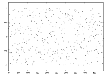
Distribution of random numbers visualized
N = 500  # no of samples
x = range(N)
y = [random.uniform(-1,1) for i in x]
from scitools.std import plot
plot(x, y, '+', axis=[0,N-1,-1.2,1.2])
Vectorized drawing of random numbers
-
random.random()generates one number at a time -
numpyhas arandommodule that efficiently generates a (large) number of random numbers at a time
from numpy import random
r = random.random()            # one no between 0 and 1
r = random.random(size=10000)  # array with 10000 numbers
r = random.uniform(-1, 10)     # one no between -1 and 10
r = random.uniform(-1, 10, size=10000)  # array
- Vectorized drawing is important for speeding up programs!
- Possible problem: two
randommodules, one Python "built-in" and one innumpy(np) - Convention: use
random(Python) andnp.random
random.uniform(-1, 1)                 # scalar number
import numpy as np
np.random.uniform(-1, 1, 100000)      # vectorized
Drawing integers
- Quite often we want to draw an integer from \( [a,b] \) and not a real number
- Python's
randommodule andnumpy.randomhave functions for drawing uniformly distributed integers:
import random
r = random.randint(a, b)  # a, a+1, ..., b

import numpy as np
r = np.random.randint(a, b+1, N)         # b+1 is not included
r = np.random.random_integers(a, b, N)   # b is included
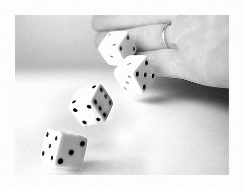
Example: Rolling a die
- Any no of eyes, 1-6, is equally probable when you roll a die
- What is the chance of getting a 6?
Rolling a die is the same as drawing integers in \( [1,6] \).
import random
N = 10000
eyes = [random.randint(1, 6) for i in range(N)]
M = 0  # counter for successes: how many times we get 6 eyes
for outcome in eyes:
    if outcome == 6:
        M += 1
print 'Got six %d times out of %d' % (M, N)
print 'Probability:', float(M)/N
Probability: M/N (exact: \( 1/6 \))
Example: Rolling a die; vectorized version
import sys, numpy as np
N = int(sys.argv[1])
eyes = np.random.randint(1, 7, N)
success = eyes == 6        # True/False array
six = np.sum(success)      # treats True as 1, False as 0
print 'Got six %d times out of %d' % (six, N)
print 'Probability:', float(M)/N
Use sum from numpy and not Python's built-in sum function! (The latter is slow, often making a vectorized version slower than the scalar version.)
Debugging programs with random numbers requires fixing the seed of the random sequence
- Debugging programs with random numbers is difficult because the numbers produced vary each time we run the program
- For debugging it is important that a new run reproduces the sequence of random numbers in the last run
- This is possible by fixing the seed of the
randommodule:
random.seed(121)(intargument)
>>> import random
>>> random.seed(2)
>>> ['%.2f' % random.random() for i in range(7)]
['0.96', '0.95', '0.06', '0.08', '0.84', '0.74', '0.67']
>>> ['%.2f' % random.random() for i in range(7)]
['0.31', '0.61', '0.61', '0.58', '0.16', '0.43', '0.39']

>>> random.seed(2)    # repeat the random sequence
>>> ['%.2f' % random.random() for i in range(7)]
['0.96', '0.95', '0.06', '0.08', '0.84', '0.74', '0.67']
By default, the seed is based on the current time
Drawing random elements from a list
There are different methods for picking an element from a list at random, but the main method applies choice(list):
>>> awards = ['car', 'computer', 'ball', 'pen']
>>> import random
>>> random.choice(awards)
'car'
Alternatively, we can compute a random index:
>>> index = random.randint(0, len(awards)-1)
>>> awards[index]
'pen'
We can also shuffle the list randomly, and then pick any element:
>>> random.shuffle(awards)
>>> awards[0]
'computer'
Example: Drawing cards from a deck; make deck and draw
# A: ace, J: jack, Q: queen, K: king
# C: clubs, D: diamonds, H: hearts, S: spades

def make_deck():
    ranks = ['A', '2', '3', '4', '5', '6', '7',
             '8', '9', '10', 'J', 'Q', 'K']
    suits = ['C', 'D', 'H', 'S']
    deck = []
    for s in suits:
        for r in ranks:
            deck.append(s + r)
    random.shuffle(deck)
    return deck

deck = make_deck()
deck = make_deck()
card = deck[0]
del deck[0]

card = deck.pop(0)  # return and remove element with index 0
Example: Drawing cards from a deck; draw a hand of cards
n cards:
def deal_hand(n, deck):
    hand = [deck[i] for i in range(n)]
    del deck[:n]
    return hand, deck
-
deckis returned since the function changes the list -
deckis changed in-place so the change affects thedeckobject in the calling code anyway, but returning changed arguments is a Python convention and good habit
Example: Drawing cards from a deck; deal
def deal(cards_per_hand, no_of_players):
    deck = make_deck()
    hands = []
    for i in range(no_of_players):
        hand, deck = deal_hand(cards_per_hand, deck)
        hands.append(hand)
    return hands

players = deal(5, 4)
import pprint; pprint.pprint(players)
[['D4', 'CQ', 'H10', 'DK', 'CK'],
 ['D7', 'D6', 'SJ', 'S4', 'C5'],
 ['C3', 'DQ', 'S3', 'C9', 'DJ'],
 ['H6', 'H9', 'C6', 'D5', 'S6']]
Example: Drawing cards from a deck; analyze results (1)
def same_rank(hand, n_of_a_kind):
    ranks = [card[1:] for card in hand]
    counter = 0
    already_counted = []
    for rank in ranks:
        if rank not in already_counted and \
               ranks.count(rank) == n_of_a_kind:
            counter += 1
            already_counted.append(rank)
    return counter
Example: Drawing cards from a deck; analyze results (2)
def same_suit(hand):
    suits = [card[0] for card in hand]
    counter = {}   # counter[suit] = how many cards of suit
    for suit in suits:
        # attention only to count > 1:
        count = suits.count(suit)
        if count > 1:
            counter[suit] = count
    return counter
Example: Drawing cards from a deck; analyze results (3)
Analysis of how many cards we have of the same suit or the same rank, with some nicely formatted printout (see the book):
The hand D4, CQ, H10, DK, CK
    has 1 pairs, 0 3-of-a-kind and
    2+2 cards of the same suit.
The hand D7, D6, SJ, S4, C5
    has 0 pairs, 0 3-of-a-kind and
    2+2 cards of the same suit.
The hand C3, DQ, S3, C9, DJ
    has 1 pairs, 0 3-of-a-kind and
    2+2 cards of the same suit.
The hand H6, H9, C6, D5, S6
    has 0 pairs, 1 3-of-a-kind and
    2 cards of the same suit.
Class implementation of a deck; class Deck
We can wrap the previous functions in a class:
- Attribute: the deck
- Methods for shuffling, dealing, putting a card back
class Deck:
    def __init__(self, shuffle=True):
        ranks = ['A', '2', '3', '4', '5', '6', '7',
                 '8', '9', '10', 'J', 'Q', 'K']
        suits = ['C', 'D', 'H', 'S']
        self.deck = [s+r for s in suits for r in ranks]
        random.shuffle(self.deck)

    def hand(self, n=1):
        """Deal n cards. Return hand as list."""
        hand = [self.deck[i] for i in range(n)]
        del self.deck[:n]

        # alternative:
        # hand = [self.pop(0) for i in range(n)]
        return hand

    def putback(self, card):
        """Put back a card under the rest."""
        self.deck.append(card)
Class implementation of a deck; alternative
class Card:
    def __init__(self, suit, rank):
        self.card = suit + str(rank)

class Hand:
    def __init__(self, list_of_cards):
        self.hand = list_of_cards

class Deck:
    def __init__(self, shuffle=True):
        ranks = ['A', '2', '3', '4', '5', '6', '7',
                 '8', '9', '10', 'J', 'Q', 'K']
        suits = ['C', 'D', 'H', 'S']
        self.deck = [Card(s,r) for s in suits for r in ranks]
        random.shuffle(self.deck)

    def deal(self, n=1):
        hand = Hand([self.deck[i] for i in range(n)])
        del self.deck[:n]
        return hand

    def putback(self, card):
        self.deck.append(card)
Class implementation of a deck; why?
To print a Deck instance, Card and Hand must have __repr__ methods that return a "pretty print" string (see the book), because print on list object applies __repr__ to print each element.
Yes! The function version has functions updating a global variable deck, as in
hand, deck = deal_hand(5, deck)
This is often considered bad programming. In the class version we avoid a global variable - the deck is stored and updated inside the class. Errors are less likely to sneak in in the class version.
Probabilities can be computed by Monte Carlo simulation
Simulate \( N \) events and count how many times \( M \) the event \( A \) happens. The probability of the event \( A \) is then \( M/N \) (as \( N\rightarrow\infty \)).
You throw two dice, one black and one green. What is the probability that the number of eyes on the black is larger than that on the green?
import random
import sys
N = int(sys.argv[1])      # no of experiments
M = 0                     # no of successful events
for i in range(N):
    black = random.randint(1, 6)   # throw black
    green = random.randint(1, 6)   # throw green
    if black > green:              # success?
        M += 1
p = float(M)/N
print 'probability:', p
A vectorized version can speed up the simulations
import sys
N = int(sys.argv[1])      # no of experiments

import numpy as np
r = np.random.random_integers(1, 6, (2, N))

black = r[0,:]            # eyes for all throws with black
green = r[1,:]            # eyes for all throws with green
success = black > green   # success[i]==True if black[i]>green[i]
M = np.sum(success)       # sum up all successes

p = float(M)/N
print 'probability:', p
Run 10+ times faster than scalar code
The exact probability can be calculated in this (simple) example
All possible combinations of two dice:
combinations = [(black, green)
                for black in range(1, 7)
                for green in range(1, 7)]
How many of the (black, green) pairs that have
the property black > green?
success = [black > green for black, green in combinations]
M = sum(success)
print 'probability:', float(M)/len(combinations)
How accurate and fast is Monte Carlo simulation?
-
black_gt_green.py: scalar version -
black_gt_green_vec.py: vectorized version -
black_gt_green_exact.py: exact version
Terminal> python black_gt_green_exact.py
probability: 0.416666666667

Terminal> time python black_gt_green.py 10000
probability: 0.4158

Terminal> time python black_gt_green.py 1000000
probability: 0.416516
real	0m1.725s

Terminal> time python black_gt_green.py 10000000
probability: 0.4164688
real	0m17.649s

Terminal> time python black_gt_green_vec.py 10000000
probability: 0.4170253
real	0m0.816s
Gamification of this example
Suppose a games is constructed such that you have to pay 1 euro to throw the two dice. You win 2 euros if there are more eyes on the black than on the green die. Should you play this game?
import sys
N = int(sys.argv[1])               # no of experiments

import random
start_capital = 10
money = start_capital
for i in range(N):
    money -= 1                     # pay for the game
    black = random.randint(1, 6)   # throw black
    green = random.randint(1, 6)   # throw brown
    if black > green:              # success?
        money += 2                 # get award

net_profit_total = money - start_capital
net_profit_per_game = net_profit_total/float(N)
print 'Net profit per game in the long run:', net_profit_per_game
Should we play the game?
Terminaldd> python black_gt_green_game.py 1000000
Net profit per game in the long run: -0.167804
No!
Vectorization of the game for speeding up the code
import sys
N = int(sys.argv[1])      # no of experiments

import numpy as np
r = np.random.random_integers(1, 6, size=(2, N))

money = 10 - N            # capital after N throws
black = r[0,:]            # eyes for all throws with black
green = r[1,:]            # eyes for all throws with green
success = black > green   # success[i] is true if black[i]>green[i]
M = np.sum(success)       # sum up all successes
money += 2*M              # add all awards for winning
print 'Net profit per game in the long run:', (money-10)/float(N)
Example: Drawing balls from a hat
We have 12 balls in a hat: four black, four red, and four blue
hat = []
for color in 'black', 'red', 'blue':
    for i in range(4):
        hat.append(color)
Choose two balls at random:
import random
index = random.randint(0, len(hat)-1)  # random index
ball1 = hat[index];  del hat[index]
index = random.randint(0, len(hat)-1)  # random index
ball2 = hat[index];  del hat[index]

# or:
random.shuffle(hat)   # random sequence of balls
ball1 = hat.pop(0)
ball2 = hat.pop(0)
What is the probability of getting two black balls or more?
def new_hat():  # make a new hat with 12 balls
    return [color for color in 'black', 'red', 'blue'
            for i in range(4)]

def draw_ball(hat):
    index = random.randint(0, len(hat)-1)
    color = hat[index];  del hat[index]
    return color, hat  # (return hat since it is modified)

# run experiments:
n = input('How many balls are to be drawn? ')
N = input('How many experiments? ')
M = 0  # no of successes

for e in range(N):
    hat = new_hat()
    balls = []         # the n balls we draw
    for i in range(n):
        color, hat = draw_ball(hat)
        balls.append(color)
    if balls.count('black') >= 2:  # two black balls or more?
        M += 1
print 'Probability:', float(M)/N
Examples on computing the probabilities
Terminal> python balls_in_hat.py
How many balls are to be drawn? 2
How many experiments? 10000
Probability: 0.0914

Terminal> python balls_in_hat.py
How many balls are to be drawn? 8
How many experiments? 10000
Probability: 0.9346

Terminal> python balls_in_hat.py
How many balls are to be drawn? 4
How many experiments? 10000
Probability: 0.4033
Guess a number game
Let the computer pick a number at random. You guess at the number, and the computer tells if the number is too high or too low.
import random
number = random.randint(1, 100)   # the computer's secret number
attempts = 0   # no of attempts to guess the number
guess = 0      # user's guess at the number
while guess != number:
    guess = input('Guess a number: ')
    attempts += 1
    if guess == number:
        print 'Correct! You used', attempts, 'attempts!'
        break
    elif guess < number:  print 'Go higher!'
    else:                 print 'Go lower!'
Monte Carlo integration
|
|
|
There is a strong link between an integral and the average of the integrand
Recall a famous theorem from calculus: Let \( f_m \) be the mean value of \( f(x) \) on \( [a,b] \). Then
$$ \int_a^b f(x)dx = f_m(b-a)$$
Idea: compute \( f_m \) by averaging \( N \) function values. To choose the \( N \) coordinates \( x_0,\ldots,x_{N-1} \) we use random numbers in \( [a,b] \). Then
$$ f_m = N^{-1}\sum_{j=0}^{N-1} f(x_j) $$
This is called Monte Carlo integration.
Implementation of Monte Carlo integration; scalar version
def MCint(f, a, b, n):
    s = 0
    for i in range(n):
        x = random.uniform(a, b)
        s += f(x)
    I = (float(b-a)/n)*s
    return I
Implementation of Monte Carlo integration; vectorized version
def MCint_vec(f, a, b, n):
    x = np.random.uniform(a, b, n)
    s = np.sum(f(x))
    I = (float(b-a)/n)*s
    return I
Monte Carlo integration is slow for \( \int f(x)dx \) (slower than the Trapezoidal rule, e.g.), but very efficient for integrating functions of many variables \( \int f(x_1,x_2,\ldots,x_n)dx_1dx_2\cdots dx_n \)
Dart-inspired Monte Carlo integration
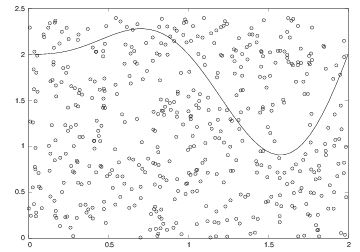
- Choose a box \( B=[x_L,x_H]\times[y_L,y_H] \) with some geometric object \( G \) inside, what is the area of \( G \)?
- Method: draw \( N \) points at random inside \( B \), count how many, \( M \), that fall within \( G \), \( G \)'s area is then \( M/N\times\hbox{area}(B) \)
- Special case: \( G \) is the geometry between \( y=f(x) \) and the \( x \) axis for \( x\in [a,b] \), i.e., the area of \( G \) is \( \int_a^bf(x)dx \), and our method gives \( \int_a^bf(x)dx \approx {M\over N}m(b-a) \) if \( B \) is the box \( [a,b]\times [0,m] \)
The code for the dart-inspired Monte Carlo integration
def MCint_area(f, a, b, n, fmax):
    below = 0  # counter for no of points below the curve
    for i in range(n):
        x = random.uniform(a, b)
        y = random.uniform(0, fmax)
        if y <= f(x):
            below += 1
    area = below/float(n)*(b-a)*fmax
    return area
from numpy import *

def MCint_area_vec(f, a, b, n, fmax):
    x = np.random.uniform(a, b, n)
    y = np.random.uniform(0, fmax, n)
    below = y[y < f(x)].size
    area = below/float(n)*(b-a)*fmax
    return area
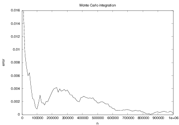
The development of the error in Monte Carlo integration
Random walk
|
|
|


Random walk in one space dimension
- One particle moves to the left and right with equal probability
- \( n \) particles start at \( x=0 \) at time \( t=0 \) - how do the particles get distributed over time?
- molecular motion
- heat transport
- quantum mechanics
- polymer chains
- population genetics
- brain research
- hazard games
- pricing of financial instruments
Program for 1D random walk
from scitools.std import plot
import random

np = 4                 # no of particles
ns = 100               # no of steps
positions = zeros(np)  # all particles start at x=0
HEAD = 1;  TAIL = 2    # constants
xmax = sqrt(ns); xmin = -xmax   # extent of plot axis

for step in range(ns):
    for p in range(np):
        coin = random_.randint(1,2)  # flip coin
        if coin == HEAD:
            positions[p] += 1   # step to the right
        elif coin == TAIL:
            positions[p] -= 1   # step to the left
    plot(positions, y, 'ko3',
         axis=[xmin, xmax, -0.2, 0.2])
    time.sleep(0.2)             # pause between moves
Random walk as a difference equation
Let \( x_n \) be the position of one particle at time \( n \). Updating rule:
$$ x_n = x_{n-1} + s$$
where \( s=1 \) or \( s=-1 \), both with probability 1/2.
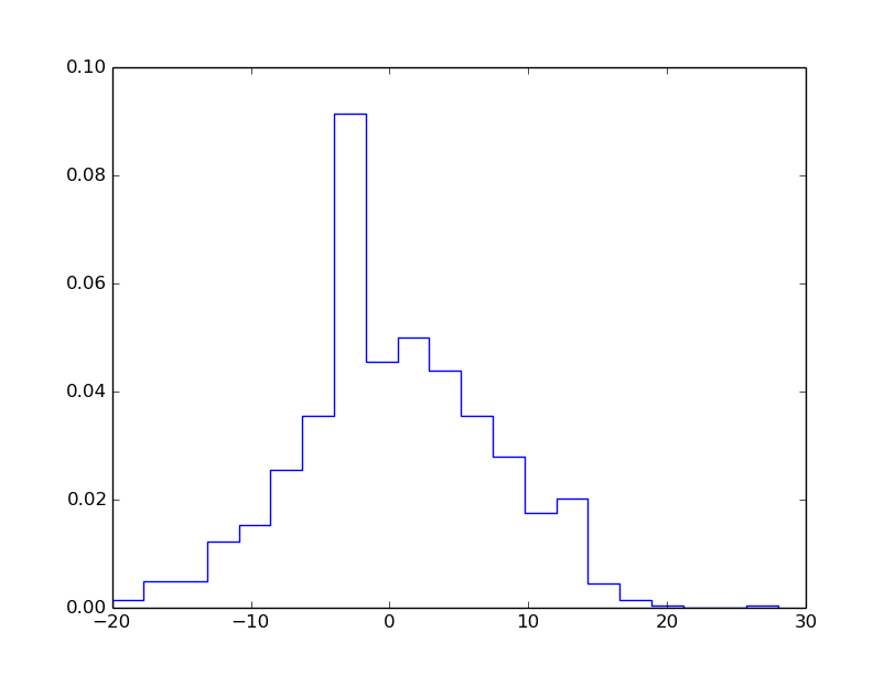
Computing statistics of the random walk
Scientists are not interested in just looking at movies of random walks - they are interested in statistics (mean position, "width" of the cluster of particles, how particles are distributed)
mean_pos  = mean(positions)
stdev_pos = std(positions)   # "width" of particle cluster

# shape of particle cluster:
from scitools.std import compute_histogram
pos, freq = compute_histogram(positions, nbins=int(xmax),
                              piecewise_constant=True)
plot(pos, freq, 'b-')
Vectorized implementation of 1D random walk
First we draw all moves at all times:
moves = numpy.random.random_integers(1, 2, size=np*ns)
moves = 2*moves - 3  #  -1, 1 instead of 1, 2
moves.shape = (ns, np)
Evolution through time:
positions = numpy.zeros(np)
for step in range(ns):
    positions += moves[step, :]

    # can do some statistics:
    print numpy.mean(positions), numpy.std(positions)
Now to more exciting stuff: 2D random walk
Let each particle move north, south, west, or east - each with probability 1/4
def random_walk_2D(np, ns, plot_step):
    xpositions = numpy.zeros(np)
    ypositions = numpy.zeros(np)
    NORTH = 1;  SOUTH = 2;  WEST = 3;  EAST = 4

    for step in range(ns):
        for i in range(len(xpositions)):
            direction = random.randint(1, 4)
            if direction == NORTH:
                ypositions[i] += 1
            elif direction == SOUTH:
                ypositions[i] -= 1
            elif direction == EAST:
                xpositions[i] += 1
            elif direction == WEST:
                xpositions[i] -= 1
    return xpositions, ypositions
Vectorized implementation of 2D random walk
def random_walk_2D(np, ns, plot_step):
    xpositions = zeros(np)
    ypositions = zeros(np)
    moves = numpy.random.random_integers(1, 4, size=ns*np)
    moves.shape = (ns, np)
    NORTH = 1;  SOUTH = 2;  WEST = 3;  EAST = 4

    for step in range(ns):
        this_move = moves[step,:]
        ypositions += where(this_move == NORTH, 1, 0)
        ypositions -= where(this_move == SOUTH, 1, 0)
        xpositions += where(this_move == EAST,  1, 0)
        xpositions -= where(this_move == WEST,  1, 0)
    return xpositions, ypositions
Visualization of 2D random walk
- We plot every
plot_stepstep - One plot on the screen + one hardcopy for movie file
- Extent of axis: it can be shown that after \( n_s \) steps, the typical width of the cluster of particles (standard deviation) is of order \( \sqrt{n_s} \), so we can set min/max axis extent as, e.g.,
xymax = 3*sqrt(ns); xymin = -xymax
Inside for loop over steps:
# just plot every plot_step steps:
if (step+1) % plot_step == 0:
    plot(xpositions, ypositions, 'ko',
         axis=[xymin, xymax, xymin, xymax],
         title='%d particles after %d steps' % \
               (np, step+1),
         savefig='tmp_%03d.png' % (step+1))
Class implementation of 2D random walk
- Can classes be used to implement a random walk?
- Yes, it sounds natural with class
Particle, holding the position of a particle as attributes and with a methodmovefor moving the particle one step - Class
Particlesholds a list ofParticleinstances and has a methodmovefor moving all particles one step and a methodmovesfor moving all particles through all steps - Additional methods in class
Particlescan plot and compute statistics - Downside: with class
Particlethe code is scalar - a vectorized versionmustuse arrays inside classParticlesinstead of a list ofParticleinstances - The implementation is an exercise
Summary of drawing random numbers (scalar code)
Draw a uniformly distributed random number in \( [0,1) \):
import random
r = random.random()
Draw a uniformly distributed random number in \( [a,b) \):
r = random.uniform(a, b)
Draw a uniformly distributed random integer in \( [a,b] \):
i = random.randint(a, b)
Summary of drawing random numbers (vectorized code)
Draw \( n \) uniformly distributed random numbers in \( [0,1) \):
import numpy as np
r = np.random.random(n)
Draw \( n \) uniformly distributed random numbers in \( [a,b) \):
r = np.random.uniform(a, b, n)
Draw \( n \) uniformly distributed random integers in \( [a,b] \):
i = np.random.randint(a, b+1, n)
i = np.random.random_integers(a, b, n)
Summary of probability computations
- Probability: perform \( N \) experiments, count \( M \) successes, then success has probability \( M/N \) (\( N \) must be large)
- Monte Carlo simulation: let a program do \( N \) experiments and count \( M \) (simple method for probability problems)
Example: investment with random interest rate
Recall difference equation for the development of an investment \( x_0 \) with annual interest rate \( p \):
$$ x_{n} = x_{n-1} + {p\over 100}x_{n-1},\quad \hbox{given }x_0$$
But:
- In reality, \( p \) is uncertain in the future
- Let us model this uncertainty by letting \( p \) be random
Assume the interest is added every month:
$$ x_{n} = x_{n-1} + {p\over 100\cdot 12}x_{n-1}$$
where \( n \) counts months
The model for changing the interest rate
\( p \) changes from one month to the next by \( \gamma \):
$$ p_n = p_{n-1} + \gamma$$
where \( \gamma \) is random
- With probability \( 1/M \), \( \gamma \neq 0 \)
(i.e., the annual interest rate changes on average every \( M \) months) - If \( \gamma\neq 0 \), \( \gamma =\pm m \), each with probability \( 1/2 \)
- It does not make sense to have \( p_n < 1 \) or \( p_n > 15 \)
The complete mathematical model
$$
\begin{align*}
x_n &= x_{n-1} + {p_{n-1}\over 12\cdot 100}x_{n-1},\quad i=1,\ldots,N\\
r_1 &= \hbox{random number in } 1,\ldots,M\\
r_2 &= \hbox{random number in } 1, 2\\
\gamma &= \left\lbrace\begin{array}{ll} m, & \hbox{if } r_1 = 1 \hbox{ and } r_2=1,\\
-m, & \hbox{if } r_1 = 1 \hbox{ and } r_2=2,\\
0, & \hbox{if } r_1 \neq 1
\end{array}\right.\\
p_n &= p_{n-1} + \left\lbrace\begin{array}{ll} \gamma, & \hbox{if } p_n+\gamma\in [1,15],\\
0, & \hbox{otherwise}
\end{array}\right.
\end{align*}
$$
A particular realization \( x_n, p_n \), \( n=0,1,\ldots,N \), is called a path (through time) or a realization. We are interested in the statistics of many paths.
Note: this is almost a random walk for the interest rate
The development of \( p \) is like a random walk, but the "particle" moves at each time level with probability \( 1/M \) (not 1 - always - as in a normal random walk).
Simulating the investment development; one path
def simulate_one_path(N, x0, p0, M, m):
    x = zeros(N+1)
    p = zeros(N+1)
    index_set = range(0, N+1)

    x[0] = x0
    p[0] = p0

    for n in index_set[1:]:
        x[n] = x[n-1] + p[n-1]/(100.0*12)*x[n-1]

        # update interest rate p:
        r = random.randint(1, M)
        if r == 1:
            # adjust gamma:
            r = random.randint(1, 2)
            gamma = m if r == 1 else -m
        else:
            gamma = 0
        pn = p[n-1] + gamma
        p[n] = pn if 1 <= pn <= 15 else p[n-1]
    return x, p
Simulating the investment development; \( N \) paths
Compute \( N \) paths (investment developments \( x_n \)) and their mean path (mean development)
def simulate_n_paths(n, N, L, p0, M, m):
    xm = zeros(N+1)
    pm = zeros(N+1)
    for i in range(n):
        x, p = simulate_one_path(N, L, p0, M, m)
        # accumulate paths:
        xm += x
        pm += p
    # compute average:
    xm /= float(n)
    pm /= float(n)
    return xm, pm
Can also compute the standard deviation path ("width" of the \( N \) paths), see the book for details
Input and graphics
Here is a list of variables that constitute the input:
x0 = 1        # initial investment
p0 = 5        # initial interest rate
N = 10*12     # number of months
M = 3         # p changes (on average) every M months
n = 1000      # number of simulations
m = 0.5       # adjustment of p
We may add some graphics in the program:
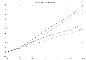
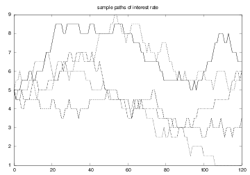
- plot some realizations of \( x_n \) and \( p_n \)
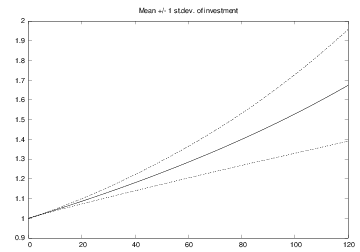
- plot the mean \( x_n \) with plus/minus one standard deviation
- plot the mean \( p_n \) with plus/minus one standard deviation
See the book for graphics details (good example on updating several different plots simultaneously in a simulation)
Some realizations of the investment
Some realizations of the interest rate
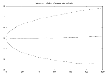
The mean and uncertainty of the investment over time
The mean and uncertainty of the interest rate over time