App.E: Programming of differential equations
Aug 21, 2016
How to solve any ordinary scalar differential equation
|
|
|
Examples on scalar differential equations (ODEs)
- Scalar ODE: a single ODE, one unknown function
- Vector ODE or systems of ODEs: several ODEs, several unknown functions
$$
\begin{align*}
u'&=\alpha u\quad\hbox{exponential growth}\\
u'&=\alpha u\left( 1-\frac{u}{R}\right)\quad\hbox{logistic growth}\\
u' + b|u|u &= g\quad\hbox{falling body in fluid}
\end{align*}
$$
We shall write an ODE in a generic form: \( u'=f(u,t) \)
- Our methods and software should be applicable to any ODE
- Therefore we need an abstract notation for an arbitrary ODE
$$ u^{\prime}(t) = f(u(t), t)$$
The three ODEs on the last slide correspond to
$$
\begin{align*}
f(u,t) &= \alpha u,\quad\hbox{exponential growth}\\
f(u,t) &= \alpha u\left( 1-\frac{u}{R}\right),\quad\hbox{logistic growth}\\
f(u,t) &= -b|u|u + g,\quad\hbox{body in fluid}
\end{align*}
$$
Our task: write functions and classes that take \( f \) as input and produce \( u \) as output
What is the \( f(u,t) \)?
Given an ODE,
$$ \sqrt{u}u' - \alpha(t) u^{3/2}(1-\frac{u}{R(t)}) = 0,$$
what is the \( f(u,t) \)?
The target form is \( u'=f(u,t) \), so we need to isolate \( u' \) on the left-hand side:
$$ u' = \underbrace{\alpha(t) u(1-\frac{u}{R(t)})}_{f(u,t)} $$
Such abstract \( f \) functions are widely used in mathematics
- Numerical differentiation: \( f'(x) \)
- Numerical integration: \( \int_a^b f(x)dx \)
- Numerical solution of algebraic equations: \( f(x)=0 \)
- \( \frac{d}{dx} x^a\sin (wx) \): \( f(x)=x^a\sin (wx) \)
- \( \int_{-1}^1 (x^2\tanh^{-1}x - (1+x^2)^{-1})dx \): \( f(x)=x^2\tanh^{-1}x - (1+x^2)^{-1} \), \( a=-1 \), \( b=1 \)
- Solve \( x^4\sin x = \tan x \): \( f(x)=x^4\sin x - \tan x \)
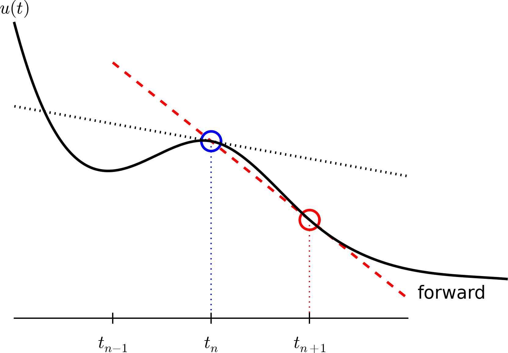
We use finite difference approximations to derivatives to turn an ODE into a difference equation
Assume we have computed \( u \) at discrete time points \( t_0,t_1,\ldots,t_k \). At \( t_k \) we have the ODE
$$ u'(t_k) = f(u(t_k),t_k) $$
Approximate \( u'(t_k) \) by a forward finite difference,
$$ u'(t_k)\approx \frac{u(t_{k+1})-u(t_k)}{\Delta t}$$
Insert in the ODE at \( t=t_k \):
$$ \frac{u(t_{k+1})-u(t_k)}{\Delta t} = f(u(t_k),t_k) $$
Terms with \( u(t_k) \) are known, and this is an algebraic (difference) equation for \( u(t_{k+1}) \)
The Forward Euler (or Euler's) method; idea
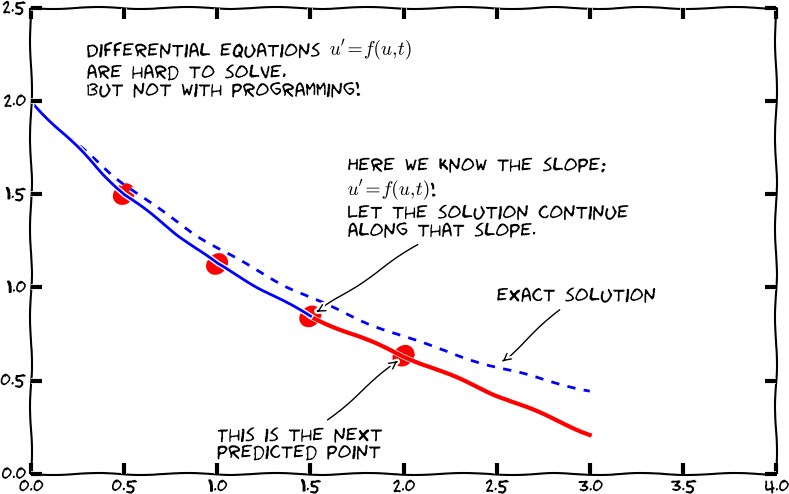
The Forward Euler (or Euler's) method; idea
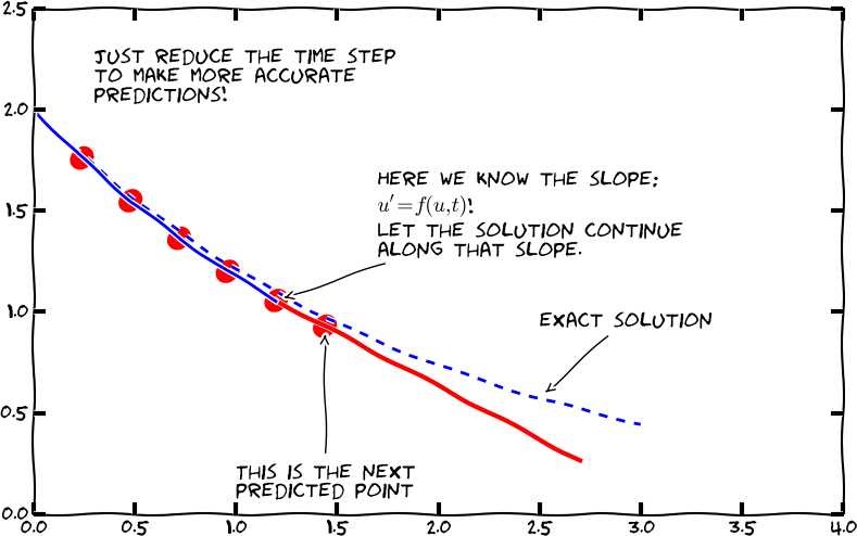
The Forward Euler (or Euler's) method; mathematics
Solving with respect to \( u(t_{k+1}) \)
$$ u(t_{k+1}) = u(t_k) + \Delta t f(u(t_k), t_k)$$
This is a very simple formula that we can use repeatedly for \( u(t_1) \), \( u(t_2) \), \( u(t_3) \) and so forth.
Let \( u_k \) denote the numerical approximation to the exact solution \( u(t) \) at \( t=t_k \).
$$ u_{k+1} = u_k + \Delta t f(u_k,t_k)$$
This is an ordinary difference equation we can solve!
Illustration of the forward finite difference
Let's apply the method!
$$ u' = u,\quad t\in (0,T] $$
Solve for \( u \) at \( t=t_k=k\Delta t \), \( k=0,1,2,\ldots,t_n \), \( t_0=0 \), \( t_n=T \)
$$ u_{k+1} = u_k + \Delta t\, f(u_k,t_k)$$
What is \( f \)? \( f(u,t)=u \)
$$ u_{k+1} = u_k + \Delta t f(u_k,t_k) = u_k + \Delta t u_k = (1+\Delta t)u_k$$
First step:
$$ u_1 = (1+\Delta t) u_0$$
but what is \( u_0 \)?
An ODE needs an initial condition: \( u(0)=U_0 \)
Any ODE \( u'=f(u,t) \) must have an initial condition \( u(0)=U_0 \), with known \( U_0 \), otherwise we cannot start the method!
In mathematics: \( u(0)=U_0 \) must be specified to get a unique solution.
$$ u'=u $$
Solution: \( u=Ce^t \) for any constant \( C \). Say \( u(0)=U_0 \): \( u=U_0e^t \).
We continue solution by hand
Say \( U_0=2 \):
$$
\begin{align*}
u_1 &= (1+\Delta t) u_0 = (1+\Delta t) U_0 = (1+\Delta t)2 \\
u_2 &= (1+\Delta t) u_1 = (1+\Delta t) (1+\Delta t)2 = 2(1+\Delta t)^2\\
u_3 &= (1+\Delta t) u_2 = (1+\Delta t) 2(1+\Delta t)^2 = 2(1+\Delta t)^3\\
u_4 &= (1+\Delta t) u_3 = (1+\Delta t) 2(1+\Delta t)^3 = 2(1+\Delta t)^4\\
u_5 &= (1+\Delta t) u_4 = (1+\Delta t) 2(1+\Delta t)^4 = 2(1+\Delta t)^5\\
\vdots &= \vdots\\
u_k &= 2(1+\Delta t)^k
\end{align*}
$$
Actually, we found a formula for \( u_k \)! No need to program...
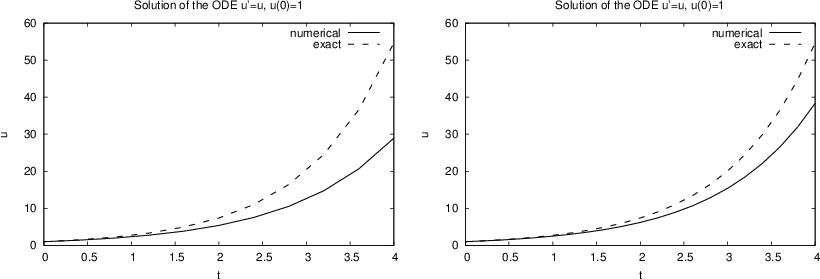
How accurate is our numerical method?
- Exact solution: \( u(t)=2e^t \), \( u(t_k)=2e^{k\Delta t} = 2(e^{\Delta t})^k \)
- Numerical solution: \( u_k = 2(1+\Delta t)^k \)
When going from \( t_k \) to \( t_{k+1} \), the solution is amplified by a factor:
- Exact: \( u(t_{k+1}) = e^{\Delta t}u(t_k) \)
- Numerical: \( u_{k+1} = (1+\Delta t)u_k \)
Using Taylor series for \( e^x \) we see that
$$ e^{\Delta t} - (1+\Delta t) = 1 + \Delta t + \frac{\Delta t^2}{2}
+ frac{\Delta t^3}{6} + \cdots - (1+\Delta t) = frac{\Delta t^3}{6}
+ {\cal O}(\Delta t^4)$$
This error approaches 0 as \( \Delta t\rightarrow 0 \).
What about the general case \( u'=f(u,t) \)?
Given any \( U_0 \):
$$
\begin{align*}
u_1 &= u_0 + \Delta t f(u_0, t_0)\\
u_2 &= u_1 + \Delta t f(u_1, t_1)\\
u_3 &= u_2 + \Delta t f(u_2, t_2)\\
u_4 &= u_3 + \Delta t f(u_3, t_3)\\
&\vdots
\end{align*}
$$
No general formula in this case...
When hand calculations get boring, let's program!
We start with a specialized program for \( u'=u \), \( u(0)=U_0 \)
Given \( \Delta t \) (dt) and \( n \)
- Create arrays
tanduof length \( n+1 \) - Set initial condition:
u[0]= \( U_0 \),t[0]=0 - For \( k=0,1,2,\ldots,n-1 \):
-
t[k+1] = t[k] + dt -
u[k+1] = (1 + dt)*u[k]
We start with a specialized program for \( u'=u \), \( u(0)=U_0 \)
import numpy as np
import sys

dt = float(sys.argv[1])
U0 = 1
T = 4
n = int(T/dt)

t = np.zeros(n+1)
u = np.zeros(n+1)

t[0] = 0
u[0] = U0
for k in range(n):
    t[k+1] = t[k] + dt
    u[k+1] = (1 + dt)*u[k]

# plot u against t
The solution if we plot \( u \) against \( t \)
\( \Delta t = 0.4 \) and \( \Delta t=0.2 \):
The algorithm for the general ODE \( u'=f(u,t) \)
Given \( \Delta t \) (dt) and \( n \)
- Create arrays
tanduof length \( n+1 \) - Create array
uto hold \( u_k \) and - Set initial condition:
u[0]= \( U_0 \),t[0]=0 - For \( k=0,1,2,\ldots,n-1 \):
-
u[k+1] = u[k] + dt*f(u[k], t[k])(the only change!) -
t[k+1] = t[k] + dt
Implementation of the general algorithm for \( u'=f(u,t) \)
def ForwardEuler(f, U0, T, n):
    """Solve u'=f(u,t), u(0)=U0, with n steps until t=T."""
    import numpy as np
    t = np.zeros(n+1)
    u = np.zeros(n+1)  # u[k] is the solution at time t[k]

    u[0] = U0
    t[0] = 0
    dt = T/float(n)

    for k in range(n):
        t[k+1] = t[k] + dt
        u[k+1] = u[k] + dt*f(u[k], t[k])

    return u, t
This simple function can solve any ODE (!)
Example on using the function
Solve \( u'=u \), \( u(0)=1 \), for \( t\in [0,4] \),
with \( \Delta t = 0.4 \)
Exact solution: \( u(t)=e^t \).
def f(u, t):
    return u

U0 = 1
T = 3
n = 30
u, t = ForwardEuler(f, U0, T, n)
from scitools.std import plot, exp
u_exact = exp(t)
plot(t, u, 'r-', t, u_exact, 'b-',
     xlabel='t', ylabel='u', legend=('numerical', 'exact'),
     title="Solution of the ODE u'=u, u(0)=1")
Now you can solve any ODE!
- Identify \( f(u,t) \) in your ODE
- Make sure you have an initial condition \( U_0 \)
- Implement the \( f(u,t) \) formula in a Python function
f(u, t) - Choose \( \Delta t \) or no of steps \( n \)
- Call
u, t = ForwardEuler(f, U0, T, n) -
plot(t, u)
The Forward Euler method may give very inaccurate solutions if \( \Delta t \) is not sufficiently small. For some problems (like \( u''+u=0 \)) other methods should be used.
Let us make a class instead of a function for solving ODEs
method = ForwardEuler(f, dt)
method.set_initial_condition(U0, t0)
u, t = method.solve(T)
plot(t, u)
- Store \( f \), \( \Delta t \), and the sequences \( u_k \), \( t_k \) as attributes
- Split the steps in the
ForwardEulerfunction into four methods: - the constructor (
__init__) -
set_initial_conditionfor \( u(0)=U_0 \) -
solvefor running the numerical time stepping -
advancefor isolating the numerical updating formula
(new numerical methods just need a differentadvancemethod, the rest is the same)
The code for a class for solving ODEs (part 1)
import numpy as np

class ForwardEuler_v1:
    def __init__(self, f, dt):
        self.f, self.dt = f, dt

    def set_initial_condition(self, U0):
        self.U0 = float(U0)
The code for a class for solving ODEs (part 2)
class ForwardEuler_v1:
    ...
    def solve(self, T):
        """Compute solution for 0 <= t <= T."""
        n = int(round(T/self.dt))  # no of intervals
        self.u = np.zeros(n+1)
        self.t = np.zeros(n+1)
        self.u[0] = float(self.U0)
        self.t[0] = float(0)

        for k in range(self.n):
            self.k = k
            self.t[k+1] = self.t[k] + self.dt
            self.u[k+1] = self.advance()
        return self.u, self.t

    def advance(self):
        """Advance the solution one time step."""
        # Create local variables to get rid of "self." in
        # the numerical formula
        u, dt, f, k, t = self.u, self.dt, self.f, self.k, self.t

        unew = u[k] + dt*f(u[k], t[k])
        return unew
Alternative class code for solving ODEs (part 1)
# Idea: drop dt in the constructor.
# Let the user provide all time points (in solve).

class ForwardEuler:
    def __init__(self, f):

        # test that f is a function
        if not callable(f):
            raise TypeError('f is %s, not a function' % type(f))
        self.f = f

    def set_initial_condition(self, U0):
        self.U0 = float(U0)

    def solve(self, time_points):
        ...
Alternative class code for solving ODEs (part 2)
class ForwardEuler:
    ...
    def solve(self, time_points):
        """Compute u for t values in time_points list."""
        self.t = np.asarray(time_points)
        self.u = np.zeros(len(time_points))

        self.u[0] = self.U0

        for k in range(len(self.t)-1):
            self.k = k
            self.u[k+1] = self.advance()
        return self.u, self.t

    def advance(self):
        """Advance the solution one time step."""
        u, f, k, t = self.u, self.f, self.k, self.t

        dt = t[k+1] - t[k]
        unew = u[k] + dt*f(u[k], t[k])
        return unew
Verifying the class implementation; mathematics
Important result: the numerical method (and most others) will exactly reproduce \( u \) if it is linear in \( t \) (!):
$$
\begin{align*}
u(t) &= at+b = 0.2t + 3\\
h(t) &= u(t)\\
u'(t) &=0.2 + (u-h(t))^4,\quad u(0)=3,\quad t\in [0,3]
\end{align*}
$$
This \( u \) should be reproduced to machine precision for any \( \Delta t \).
Verifying the class implementation; implementation
def test_ForwardEuler_against_linear_solution():
    def f(u, t):
        return 0.2 + (u - h(t))**4

    def h(t):
        return 0.2*t + 3

    solver = ForwardEuler(f)
    solver.set_initial_condition(U0=3)
    dt = 0.4; T = 3; n = int(round(float(T)/dt))
    time_points = np.linspace(0, T, n+1)
    u, t = solver.solve(time_points)
    u_exact = h(t)
    diff = np.abs(u_exact - u).max()
    tol = 1E-14
    success = diff < tol
    assert success
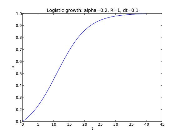
Using a class to hold the right-hand side \( f(u,t) \)
$$ u^{\prime}(t)=\alpha u(t)\left( 1-\frac{u(t)}{R}\right),\quad u(0)=U_0,\quad t\in [0,40]$$
class Logistic:
    def __init__(self, alpha, R, U0):
        self.alpha, self.R, self.U0 = alpha, float(R), U0

    def __call__(self, u, t):   # f(u,t)
        return self.alpha*u*(1 - u/self.R)
problem = Logistic(0.2, 1, 0.1)
time_points = np.linspace(0, 40, 401)
method = ForwardEuler(problem)
method.set_initial_condition(problem.U0)
u, t = method.solve(time_points)
Figure of the solution
Numerical methods for ordinary differential equations
$$ u_{k+1} = u_k + \Delta t\, f(u_k, t_k) $$
$$ u_{k+1} = u_k + {1\over 6}\left( K_1 + 2K_2 + 2K_3 + K_4\right)$$
$$
\begin{align*}
K_1 &= \Delta t\,f(u_k, t_k)\\
K_2 &= \Delta t\,f(u_k + {1\over2}K_1, t_k + {1\over2}\Delta t)\\
K_3 &= \Delta t\,f(u_k + {1\over2}K_2, t_k + {1\over2}\Delta t)\\
K_4 &= \Delta t\,f(u_k + K3, t_k + \Delta t)
\end{align*}
$$
And lots of other methods! How to program a wide collection of methods? Use object-oriented programming!
A superclass for ODE methods
- Store the solution \( u_k \) and the corresponding time levels \( t_k \), \( k=0,1,2,\ldots,n \)
- Store the right-hand side function \( f(u,t) \)
- Set and store the initial condition
- Run the loop over all time steps
- Common data and functionality are placed in superclass
ODESolver - Isolate the numerical updating formula in a method
advance - Subclasses, e.g.,
ForwardEuler, just implement the specific numerical formula inadvance
The superclass code
class ODESolver:
    def __init__(self, f):
        self.f = f

    def advance(self):
        """Advance solution one time step."""
        raise NotImplementedError  # implement in subclass

    def set_initial_condition(self, U0):
        self.U0 = float(U0)

    def solve(self, time_points):
        self.t = np.asarray(time_points)
        self.u = np.zeros(len(self.t))
        # Assume that self.t[0] corresponds to self.U0
        self.u[0] = self.U0

        # Time loop
        for k in range(n-1):
            self.k = k
            self.u[k+1] = self.advance()
        return self.u, self.t

    def advance(self):
        raise NotImplemtedError # to be impl. in subclasses
Implementation of the Forward Euler method
class ForwardEuler(ODESolver):
    def advance(self):
        u, f, k, t = self.u, self.f, self.k, self.t

        dt = t[k+1] - t[k]
        unew = u[k] + dt*f(u[k], t)
        return unew
from ODESolver import ForwardEuler
def test1(u, t):
    return u

method = ForwardEuler(test1)
method.set_initial_condition(U0=1)
u, t = method.solve(time_points=np.linspace(0, 3, 31))
plot(t, u)
The implementation of a Runge-Kutta method
class RungeKutta4(ODESolver):
    def advance(self):
        u, f, k, t = self.u, self.f, self.k, self.t

        dt = t[k+1] - t[k]
        dt2 = dt/2.0
        K1 = dt*f(u[k], t)
        K2 = dt*f(u[k] + 0.5*K1, t + dt2)
        K3 = dt*f(u[k] + 0.5*K2, t + dt2)
        K4 = dt*f(u[k] + K3, t + dt)
        unew = u[k] + (1/6.0)*(K1 + 2*K2 + 2*K3 + K4)
        return unew
from ODESolver import RungeKutta4
def test1(u, t):
    return u

method = RungeKutta4(test1)
method.set_initial_condition(U0=1)
u, t = method.solve(time_points=np.linspace(0, 3, 31))
plot(t, u)
The user should be able to check intermediate solutions and terminate the time stepping
- Sometimes a property of the solution determines when to stop the solution process: e.g., when \( u < 10^{-7}\approx 0 \).
- Extension:
solve(time_points, terminate) -
terminate(u, t, step_no)is called at every time step, is user-defined, and returnsTruewhen the time stepping should be terminated - Last computed solution is
u[step_no]at timet[step_no]
def terminate(u, t, step_no):
    eps = 1.0E-6                     # small number
    return abs(u[step_no,0]) < eps   # close enough to zero?
Systems of differential equations (vector ODE)
|
|
|
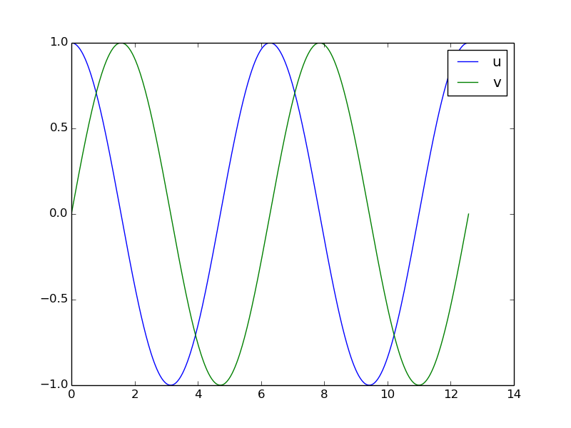
Example on a system of ODEs (vector ODE)
Two ODEs with two unknowns \( u(t) \) and \( v(t) \):
$$
\begin{align*}
u'(t) &= v(t)\\
v'(t) &= -u(t)
\end{align*}
$$
Each unknown must have an initial condition, say
$$ u(0)=0,\quad v(0)=1 $$
In this case, one can derive the exact solution to be
$$ u(t)=\sin (t),\quad v(t)=\cos (t)$$
Systems of ODEs appear frequently in physics, biology, finance, ...
The ODE system that is the final project in the course
Model for spreading of a disease in a population:
$$
\begin{align*}
S' &= - \beta SI\\
I' &= \beta SI -\nu R\\
R' &= \nu I
\end{align*}
$$
Initial conditions:
$$
\begin{align*}
S(0) &= S_0\\
I(0) &= I_0\\
R(0) &= 0
\end{align*}
$$
Another example on a system of ODEs (vector ODE)
Second-order ordinary differential equation, for a spring-mass system (from Newton's second law):
$$ mu'' + \beta u' + ku = 0,\quad u(0)=U_0,\ u'(0)=0$$
We can rewrite this as a system of two first-order equations, by introducing two new unknowns
$$ u^{(0)}(t) \equiv u(t),\quad u^{(1)}(t) \equiv u'(t)$$
The first-order system is then
$$
\begin{align*}
{d\over dt} u^{(0)}(t) &= u^{(1)}(t)\\
{d\over dt} u^{(1)}(t) &= -m^{-1}\beta u^{(1)} - m^{-1}ku^{(0)}
\end{align*}
$$
Initial conditions: \( u^{(0)}(0) = U_0 \), \( u^{(1)}(0)=0 \)
Making a flexible toolbox for solving ODEs
- For scalar ODEs we could make one general class hierarchy to solve "all" problems with a range of methods
- Can we easily extend class hierarchy to systems of ODEs?
- Yes!
- The example here can easily be extended to professional code (Odespy)
Vector notation for systems of ODEs: unknowns and equations
General software for any vector/scalar ODE demands a general mathematical notation. We introduce \( n \) unknowns
$$ u^{(0)}(t), u^{(1)}(t), \ldots, u^{(n-1)}(t) $$
in a system of \( n \) ODEs:
$$
\begin{align*}
{d\over dt}u^{(0)} &= f^{(0)}(u^{(0)}, u^{(1)}, \ldots, u^{(n-1)}, t)\\
{d\over dt}u^{(1)} &= f^{(1)}(u^{(0)}, u^{(1)}, \ldots, u^{(n-1)}, t)\\
\vdots &=& \vdots\\
{d\over dt}u^{(n-1)} &= f^{(n-1)}(u^{(0)}, u^{(1)}, \ldots, u^{(n-1)}, t)
\end{align*}
$$
Vector notation for systems of ODEs: vectors
We can collect the \( u^{(i)}(t) \) functions and right-hand side functions \( f^{(i)} \) in vectors:
$$ u = (u^{(0)}, u^{(1)}, \ldots, u^{(n-1)})$$
$$ f = (f^{(0)}, f^{(1)}, \ldots, f^{(n-1)})$$
The first-order system can then be written
$$ u' = f(u, t),\quad u(0) = U_0$$
where \( u \) and \( f \) are vectors and \( U_0 \) is a vector of initial conditions
Observe that the notation makes a scalar ODE and a system look the same, and we can easily make Python code that can handle both cases within the same lines of code (!)
How to make class ODESolver work for systems of ODEs
- Recall: ODESolver was written for a scalar ODE
- Now we want it to work for a system \( u'=f \), \( u(0)=U_0 \), where \( u \), \( f \) and \( U_0 \) are vectors (arrays)
- What are the problems?
Forward Euler applied to a system:
$$
\underbrace{u_{k+1}}_{\mbox{vector}} =
\underbrace{u_k}_{\mbox{vector}} +
\Delta t\, \underbrace{f(u_k, t_k)}_{\mbox{vector}}
$$
In Python code:
unew = u[k] + dt*f(u[k], t)
where
-
uis a two-dim. array (u[k]is a row) -
fis a function returning an array (all the right-hand sides \( f^{(0)},\ldots,f^{(n-1)} \))
The adjusted superclass code (part 1)
- Ensure that
f(u,t)returns an array.
This can be done be a general adjustment in the superclass! - Inspect \( U_0 \) to see if it is a number or list/tuple and
make corresponding
u1-dim or 2-dim array
class ODESolver:
    def __init__(self, f):
        # Wrap user's f in a new function that always
        # converts list/tuple to array (or let array be array)
        self.f = lambda u, t: np.asarray(f(u, t), float)

    def set_initial_condition(self, U0):
        if isinstance(U0, (float,int)):  # scalar ODE
            self.neq = 1                 # no of equations
            U0 = float(U0)
        else:                            # system of ODEs
            U0 = np.asarray(U0)
            self.neq = U0.size           # no of equations
        self.U0 = U0
The superclass code (part 2)
class ODESolver:
    ...
    def solve(self, time_points, terminate=None):
        if terminate is None:
            terminate = lambda u, t, step_no: False

        self.t = np.asarray(time_points)
        n = self.t.size
        if self.neq == 1:  # scalar ODEs
            self.u = np.zeros(n)
        else:              # systems of ODEs
            self.u = np.zeros((n,self.neq))

        # Assume that self.t[0] corresponds to self.U0
        self.u[0] = self.U0

        # Time loop
        for k in range(n-1):
            self.k = k
            self.u[k+1] = self.advance()
            if terminate(self.u, self.t, self.k+1):
                break  # terminate loop over k
        return self.u[:k+2], self.t[:k+2]
All subclasses from the scalar ODE works for systems as well
Example on how to use the general class hierarchy
$$ mu'' + \beta u' + ku = 0,\quad u(0),\ u'(0)\hbox{ known}$$
$$
\begin{align*}
u^{(0)} &= u,\quad u^{(1)} = u'\\
u(t) &= (u^{(0)}(t), u^{(1)}(t))\\
f(u,t)&=(u^{(1)}(t), -m^{-1}\beta u^{(1)} - m^{-1}ku^{(0)})\\
u'(t) &= f(u,t)
\end{align*}
$$
def myf(u, t):
    # u is array with two components u[0] and u[1]:
    return [u[1],
            -beta*u[1]/m - k*u[0]/m]
Alternative implementation of the \( f \) function via a class
class MyF:
    def __init__(self, m, k, beta):
        self.m, self.k, self.beta = m, k, beta

    def __call__(self, u, t):
        m, k, beta = self.m, self.k, self.beta
        return [u[1], -beta*u[1]/m - k*u[0]/m]
from ODESolver import ForwardEuler
# initial condition:
U0 = [1.0, 0]
f = MyF(1.0, 1.0, 0.0)   # u'' + u = 0 => u(t)=cos(t)
solver = ForwardEuler(f)
solver.set_initial_condition(U0)

T = 4*pi; dt = pi/20; n = int(round(T/dt))
time_points = np.linspace(0, T, n+1)
u, t = solver.solve(time_points)

# u is an array of [u0,u1] arrays, plot all u0 values:
u0_values = u[:,0]
u0_exact = cos(t)
plot(t, u0_values, 'r-',  t, u0_exact, 'b-')
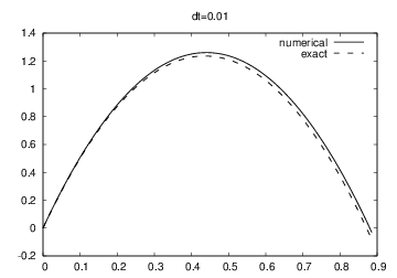
Throwing a ball; ODE model
Newton's 2nd law for a ball's trajectory through air leads to
$$
\begin{align*}
{dx\over dt} &= v_x\\
{dv_x\over dt} &= 0\\
{dy\over dt} &= v_y\\
{dv_y\over dt} &= -g
\end{align*}
$$
Air resistance is neglected but can easily be added!
- 4 ODEs with 4 unknowns:
- the ball's position \( x(t) \), \( y(t) \)
- the velocity \( v_x(t) \), \( v_y(t) \)
Throwing a ball; code
def f(u, t):
    x, vx, y, vy = u
    g = 9.81
    return [vx, 0, vy, -g]
from ODESolver import ForwardEuler
# t=0: prescribe x, y, vx, vy
x = y = 0                     # start at the origin
v0 = 5;  theta = 80*pi/180    # velocity magnitude and angle
vx = v0*cos(theta)
vy = v0*sin(theta)
# Initial condition:
U0 = [x, vx, y, vy]

solver= ForwardEuler(f)
solver.set_initial_condition(u0)
time_points = np.linspace(0, 1.2, 101)
u, t = solver.solve(time_points)

# u is an array of [x,vx,y,vy] arrays, plot y vs x:
x = u[:,0];  y = u[:,2]
plot(x, y)
Throwing a ball; results
Comparison of exact and Forward Euler solutions
Logistic growth model; ODE and code overview
$$ u' = \alpha u(1 - u/{\color{red}R(t)}),\quad u(0)=U_0 $$
\( R \) is the maximum population size,
which can vary with changes in the environment over time
- Class Problem holds "all physics": \( \alpha \), \( R(t) \), \( U_0 \), \( T \) (end time), \( f(u,t) \) in ODE
- Class Solver holds "all numerics": \( \Delta t \), solution method; solves the problem and plots the solution
- Solve for \( t\in [0,T] \) but terminate when \( |u-R| < \hbox{tol} \)
Logistic growth model; class Problem (\( f \))
class Problem:
    def __init__(self, alpha, R, U0, T):
        self.alpha, self.R, self.U0, self.T = alpha, R, U0, T

    def __call__(self, u, t):
        """Return f(u, t)."""
        return self.alpha*u*(1 - u/self.R(t))

    def terminate(self, u, t, step_no):
        """Terminate when u is close to R."""
        tol = self.R*0.01
        return abs(u[step_no] - self.R) < tol

problem = Problem(alpha=0.1, R=500, U0=2, T=130)
Logistic growth model; class Solver
class Solver:
def __init__(self, problem, dt,
method=ODESolver.ForwardEuler):
self.problem, self.dt = problem, dt
self.method = method
def solve(self):
solver = self.method(self.problem)
solver.set_initial_condition(self.problem.U0)
n = int(round(self.problem.T/self.dt))
t_points = np.linspace(0, self.problem.T, n+1)
self.u, self.t = solver.solve(t_points,
self.problem.terminate)
def plot(self):
plot(self.t, self.u)
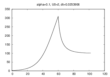
problem = Problem(alpha=0.1, U0=2, T=130,
R=lambda t: 500 if t < 60 else 100)
solver = Solver(problem, dt=1.)
solver.solve()
solver.plot()
print 'max u:', solver.u.max()
Logistic growth model; results