App. A: Sequences and difference equations

Sequences is a central topic in mathematics: $$x_0,\ x_1,\ x_2,\ \ldots,\ x_n,\ldots,$$

Example: all odd numbers $$1, 3, 5, 7, \ldots, 2n+1,\ldots$$

For this sequence we have a formula for the $n$-th term: $$x_n = 2n+1$$ and we can write the sequence more compactly as $$(x_n)_{n=0}^\infty,\quad x_n = 2n+1$$

$$1,\ 4,\ 9,\ 16,\ 25,\ \ldots\quad (x_n)_{n=0}^\infty,\ x_n=n^2$$ $$1,\ {1\over 2},\ {1\over3},\ {1\over4},\ \ldots\quad (x_n)_{n=0}^\infty,\ x_n={1\over {n+1}}$$ $$1,\ 1,\ 2,\ 6,\ 24,\ \ldots\quad (x_n)_{n=0}^\infty,\ x_n=n!$$ $$1,\ 1+x,\ 1+x+{1\over2}x^2,\ 1+x+{1\over2}x^2+{1\over6}x^3,\ \ldots\quad (x_n)_{n=0}^\infty,\ x_n=\sum_{j=0}^n {x^j\over j!}$$

• Infinite sequences have an infinite number of terms ($n\rightarrow\infty$)
• In mathematics, infinite sequences are widely used
• In real-life applications, sequences are usually finite: $(x_n)_{n=0}^N$
• Example: number of approved exercises every week in INF1100
  $x_0, x_1, x_2, \ldots, x_{15}$
• Example: the annual value of a loan
  $x_0, x_1, \ldots, x_{20}$

• For sequences occuring in modeling of real-world phenomena, there is seldom a formula for the $n$-th term
• However, we can often set up one or more equations governing the sequence
• Such equations are called difference equations
• With a computer it is then very easy to generate the sequence by solving the difference equations
• Difference equations have lots of applications and are very easy to solve on a computer, but often complicated or impossible to solve for $x_n$ (as a formula) by pen and paper!
• The programs require only loops and arrays

Put $x_0$ money in a bank at year 0. What is the value after $N$ years if the interest rate is $p$ percent per year?

The fundamental information relates the value at year $n$, $x_n$, to the value of the previous year, $x_{n-1}$: $$x_{n} = x_{n-1} + {p\over 100}x_{n-1}$$

How to solve for $x_n$? Start with $x_0$, compute $x_1$, $x_2$, ...

Solve math equations by repeating a simple procedure (relation) many times (boring, but well suited for a computer!)

• Previous program stores all the $x_n$ values in a NumPy array
• To compute $x_n$, we only need one previous value, $x_{n-1}$

x_old = x0
for n in index_set[1:]:
    x_new = x_old + (p/100.)*x_old
    x_old = x_new  # x_new becomes x_old at next step

However, programming with an array x[n] is simpler, safer, and enables plotting the sequence, so we will continue to use arrays in the examples

• A more relevant model is to add the interest every day
• The interest rate per day is $r=p/D$ if $p$ is the annual interest rate and $D$ is the number of days in a year
• A common model in business applies $D=360$, but $n$ counts exact (all) days

How can we find the number of days between two dates?

>>> import datetime
>>> date1 = datetime.date(2007, 8, 3)  # Aug 3, 2007
>>> date2 = datetime.date(2008, 8, 4)  # Aug 4, 2008
>>> diff = date2 - date1
>>> print diff.days
367

• Could not be handled in school (cannot apply $x_n =x_0(1+\frac{p}{100})^n$)
• A varying $p$ causes no problems in the program: just fill an array p with correct interest rate for day n

p = zeros(len(index_set))
# fill p[n] for n in index_set (might be non-trivial...)

r = p/360.0                      # daily interest rate
x = zeros(len(index_set))

x[0] = x0
for n in index_set[1:]:
    x[n] = x[n-1] + (r[n-1]/100.0)*x[n-1]

• A loan $L$ is paid back with a fixed amount $L/N$ every month over $N$ months + the interest rate of the loan
• $p$: annual interest rate, $p/12:$ monthly rate
• Let $x_n$ be the value of the loan at the end of month $n$

($L/N$ makes the equation nonhomogeneous)

• We have a fortune $F$ invested with an annual interest rate of $p$ percent
• Every year we plan to consume an amount $c_n$ ($n$ counts years)
• Let $x_n$ be our fortune at year $n$

Simplest possibility: keep $c_n$ constant, but inflation demands $c_n$ to increase...

• Assume $I$ percent inflation per year
• Start with $c_0$ as $q$ percent of the interest the first year
• $c_n$ then develops as money with interest rate $I$

This is a coupled system of two difference equations, but the programming is still simple: we update two arrays, first x[n], then c[n], inside the loop (good exercise!)

No programming or math course is complete without an example on Fibonacci numbers: $$x_n = x_{n-1} + x_{n-2},\quad x_0=1,\ x_1=1$$

This is a homogeneous difference equation of second order (second order means three levels: $n$, $n-1$, $n-2$). This classification is important for mathematical solution technique, but not for simulation in a program.

Run the program with $N=50$:

2 2
3 3
4 5
5 8
6 13
...
45 1836311903
Warning: overflow encountered in long_scalars
46 -1323752223

Note:

• Changing int to long or int64 for array elements allows $N\leq 91$
• Can use float96 (though $x_n$ is integer): $N \leq 23600$

• Best: use Python scalars of type int - these automatically changes to long when overflow in int
• The long type in Python has arbitrarily many digits (as many as required in a computation!)
• Note: long for arrays is 64-bit integer (int64), while scalar long in Python is an integer with as "infinitely" many digits

The program now avoids arrays and makes use of three int objects (which automatically changes to long when needed):

import sys
N = int(sys.argv[1])
xnm1 = 1                           # "x_n minus 1"
xnm2 = 1                           # "x_n minus 2"
n = 2
while n <= N:
    xn = xnm1 + xnm2
    print 'x_%d = %d' % (n, xn)
    xnm2 = xnm1
    xnm1 = xn
    n += 1

Run with $N=200$:

x_2 = 2
x_3 = 3
...
x_198 = 173402521172797813159685037284371942044301
x_199 = 280571172992510140037611932413038677189525
x_200 = 453973694165307953197296969697410619233826

Limition: your computer's memory

The model for growth of money in a bank has a solution of the type $$x_n = x_0C^n \quad (= x_0e^{n\ln C})$$

Note:

• This is exponential growth in time ($n$)
• Populations of humans, animals, and cells also exhibit the same type of growth as long as there are unlimited resources (space and food)
• Most environments can only support a maximum number $M$ of individuals
• How can we model this limitation?

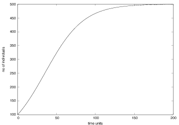
Initially, when there are enough resources, the growth is exponential: $$x_n = x_{n-1} + {r\over 100}x_{n-1}$$

The growth rate $r$ must decay to zero as $x_n$ approaches $M$. The simplest variation of $r(n)$ is a linear: $$r(n) = \varrho \left(1 - {x_n\over M}\right)$$

Observe: $r(n)\approx \varrho$ for small $n$ when $x_n\ll M$, and $r(n) \rightarrow 0$ as $x_n\rightarrow M$ and $n$ is big

$$x_n = x_{n-1} + {\varrho\over 100} x_{n-1}\left(1 - {x_{n-1}\over M}\right)$$ (This is a nonlinear difference equation)

In a program it is easy to introduce logistic instead of exponential growth, just replace

x[n] = x[n-1] + p/100.0)*x[n-1]

by

x[n] = x[n-1] + (rho/100.0)*x[n-1]*(1 - x[n-1]/float(M))

The factorial $n!$ is defined as $$n(n-1)(n-2)\cdots 1,\quad 0!=1$$

The following difference equation has $x_n=n!$ as solution and can be used to compute the factorial: $$x_n = nx_{n-1},\quad x_0 = 1$$

• In mathematics, it is much stressed that a difference equation for $x_n$ must have an initial condition $x_0$
• The initial condition is obvious when programming: otherwise we cannot start the program ($x_0$ is needed to compute $x_n$)
• However: if you forget x[0] = x0 in the program, you get $x_0=0$ (because x = zeroes(N+1)), which (usually) gives unintended results!

• How can you calculate $\sin x$, $\ln x$, $e^x$ without a calculator or program?
• These functions were originally defined to have some desired mathematical properties, but without an algorithm for how to evaluate function values
• Idea: approximate $\sin x$, etc. by polynomials, since they are easy to calculate (sum, multiplication), but how??

$$\sin x = \sum_{k=0}^\infty (-1)^k\frac{x^{2k+1}}{(2k+1)!}$$

$$f(x) = \sum_{k=0}^\infty \frac{1}{k!}(\frac{d^k}{dx^k} f(0))x^k$$ For "any" $f(x)$, if we can differentiate, add, and multiply $x^k$, we can evaluate $f$ at any $x$ (!!!)

$$f(x) \approx \sum_{k=0}^{{\color{red} N}} \frac{1}{k!}(\frac{d^k}{dx^k} f(0))x^k$$

$N=1$ is very popular and has been essential in developing physics and technology

$$\begin{align*} e^x &= \sum_{k=0}^\infty \frac{x^k}{k!}\\ &\approx 1 + x + \frac{1}{2}x^2 + \frac{1}{6}x^3\\ &\approx 1 + x \end{align*}$$

The previous Taylor polynomials are most accurate around $x=0$. Can make the polynomials accurate around any point $x=a$: $$f(x) \approx \sum_{k=0}^N \frac{1}{k!}(\frac{d^k}{dx^k} f(a))(x-a)^k$$

The Taylor series for $e^x$ around $x=0$ reads $$e^x= \sum_{n=0}^\infty {x^n\over n!}$$

Define $$e_{n}=\sum_{k=0}^{n-1} \frac{x^k}{k!} = \sum_{k=0}^{n-2} \frac{x^k}{k!} + \frac{x^{n-1}}{(n-1)!}$$

We can formulate the sum in $e_n$ as the following difference equation: $$e_n = e_{n-1} + \frac{x^{n-1}}{(n-1)!},\quad e_0=0$$

Observe: $$\frac{x^n}{n!} = \frac{x^{n-1}}{(n-1)!}\cdot \frac{x}{n}$$

Let $a_n = x^n/n!$. Then we can efficiently compute $a_n$ via $$a_n = a_{n-1}\frac{x}{n},\quad a_0 = 1$$

Now we can update each term via the $a_n$ equation and sum the terms via the $e_n$ equation: $$\begin{align*} e_n &= e_{n-1} + a_{n-1},\quad e_0 = 0,\ a_0 = 1\\ a_n &= \frac{x}{n} a_{n-1} \end{align*}$$

See the book for more details

$$f(x)=0$$

$$ax + b = 0$$ $$ax^2 + bx + c = 0$$ $$\sin x + \cos x = 1$$

• Simple numerical algorithms can solve "any" equation $f(x)=0$
• Safest: Bisection
• Fastest: Newton's method
• Don't like $f'(x)$ in Newton's method? Use the Secant method
• Secant and Newton are difference equations!

Simpson (1740) came up with the following general method for solving $f(x)=0$ (based on ideas by Newton): $$x_n = x_{n-1} - {f(x_{n-1})\over f'(x_{n-1})},\quad x_0 \hbox{ given}$$

Note:

• This is a (nonlinear!) difference equation
• As $n\rightarrow\infty$, we hope that $x_n\rightarrow x_s$, where $x_s$ solves $f(x_s)=0$
• How to choose $N$ when what we want is $x_N$ close to $x_s$?
• Need a slightly different program: simulate until $f(x)\leq \epsilon$, where $\epsilon$ is a small tolerance
• Caution: Newton's method may (easily) diverge, so $f(x)\leq\epsilon$ may never occur!

def Newton(f, x, dfdx, epsilon=1.0E-7, max_n=100):
    n = 0
    while abs(f(x)) > epsilon and n <= max_n:
        x = x - f(x)/dfdx(x)
        n += 1
    return x, n, f(x)

Note:

• $f(x)$ is evaluated twice in each pass of the loop - only one evaluation is strictly necessary (can store the value in a variable and reuse it)
• f(x)/dfdx(x) can give integer division
• It could be handy to store the x and f(x) values in each iteration (for plotting or printing a convergence table)

Only one $f(x)$ call in each iteration, optional storage of $(x,f(x))$ values during the iterations, and ensured float division:

def Newton(f, x, dfdx, epsilon=1.0E-7, max_n=100,
           store=False):
    f_value = f(x)
    n = 0
    if store: info = [(x, f_value)]
    while abs(f_value) > epsilon and n <= max_n:
        x = x - float(f_value)/dfdx(x)
        n += 1
        f_value = f(x)
        if store: info.append((x, f_value))
    if store:
        return x, info
    else:
        return x, n, f_value

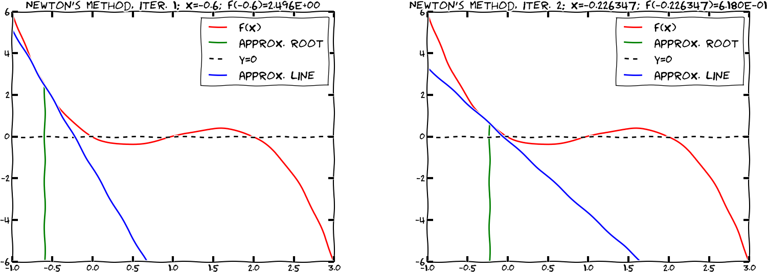
$$e^{-0.1x^2}\sin ({\pi\over 2}x) =0\] Solutions: $x=0, \pm 2, \pm 4, \pm 6, \ldots$$$

$x_0=1.7$ gives quick convergence towards the closest root $x=0$:

zero: 1.999999999768449
Iteration  0: f(1.7)=0.340044
Iteration  1: f(1.99215)=0.00828786
Iteration  2: f(1.99998)=2.53347e-05
Iteration  3: f(2)=2.43808e-10

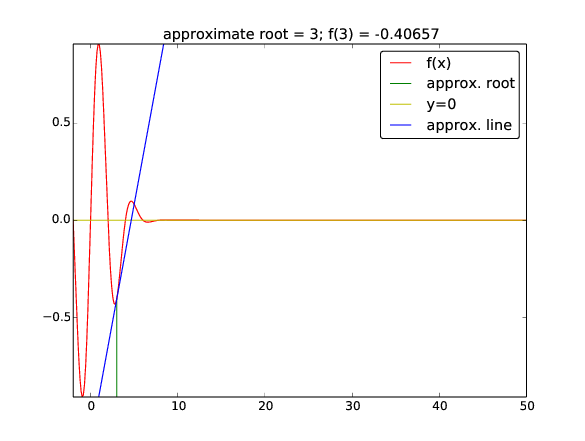
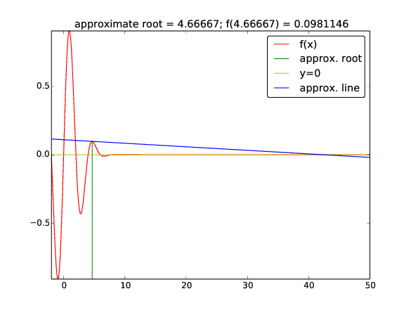
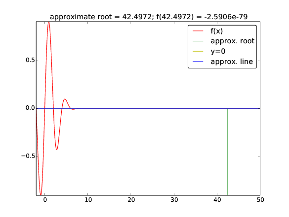
Start value $x_0=3$ (closest root $x=2$ or $x=4$):

zero: 42.49723316011362
Iteration  0: f(3)=-0.40657
Iteration  1: f(4.66667)=0.0981146
Iteration  2: f(42.4972)=-2.59037e-79

Try the demo program src/diffeq/Newton_movie.py with $x_0=3$, $x\in [-2,50]$ for plotting and numerical approximation of $f'(x)$:

Terminal> python Newton_movie.py "exp(-0.1*x**2)*sin(pi/2*x)" \
          numeric 3 -2 50

Newton's method may work fine or give wrong results! You need to understand the method to interpret the results!

A tone A (440 Hz) is a sine wave with frequency 440 Hz: $$s(t) = A\sin\left( 2\pi f t\right),\quad f = 440$$

On a computer we represent $s(t)$ by a discrete set of points on the function curve (exactly as we do when we plot $s(t)$). CD quality needs 44100 samples per second.

• $r$: sampling rate (samples per second, default 44100)
• $f$: frequency of the tone
• $m$: duration of the tone (seconds)

Code (we use descriptive names: frequency $f$, length $m$, amplitude $A$, sample_rate $r$):

import numpy
def note(frequency, length, amplitude=1,
         sample_rate=44100):
    time_points = numpy.linspace(0, length,
                                 length*sample_rate)
    data = numpy.sin(2*numpy.pi*frequency*time_points)
    data = amplitude*data
    return data

• We have data as an array with float and unit amplitude
• Sound data in a file should have 2-byte integers (int16) as data elements and amplitudes up to $2^{15}-1$ (max value for int16 data)

data = note(440, 2)
data = data.astype(numpy.int16)
max_amplitude = 2**15 - 1
data = max_amplitude*data
import scitools.sound
scitools.sound.write(data, 'Atone.wav')
scitools.sound.play('Atone.wav')

• Let us read a sound file and add echo
• Sound = array s[n]
• Echo means to add a delay of the sound

# echo: e[n] = beta*s[n] + (1-beta)*s[n-b]

def add_echo(data, beta=0.8, delay=0.002,
             sample_rate=44100):
    newdata = data.copy()
    shift = int(delay*sample_rate)  # b (math symbol)
    for i in xrange(shift, len(data)):
        newdata[i] = beta*data[i] + (1-beta)*data[i-shift]
    return newdata

Load data, add echo and play:

data = scitools.sound.read(filename)
data = data.astype(float)
data = add_echo(data, beta=0.6)
data = data.astype(int16)
scitools.sound.play(data)

• Each note is an array of samples from a sine with a frequency corresponding to the note
• Assume we have several note arrays data1, data2, ...:

# put data1, data2, ... after each other in a new array:
data = numpy.concatenate((data1, data2, data3, ...))

The start of "Nothing Else Matters" (Metallica):

E1 = note(164.81, .5)
G = note(392, .5)
B = note(493.88, .5)
E2 = note(659.26, .5)
intro = numpy.concatenate((E1, G, B, E2, B, G))
...
song = numpy.concatenate((intro, intro, ...))
scitools.sound.play(song)
scitools.sound.write(song, 'tmp.wav')

• Sequence: $x_0$, $x_1$, $x_2$, $\ldots$, $x_n$, $\ldots$, $x_N$
• Difference equation: relation between $x_n$, $x_{n-1}$ and maybe $x_{n-2}$ (or more terms in the "past") + known start value $x_0$ (and more values $x_1$, ... if more levels enter the equation)

index_set = <array of n-values: 0, 1, ..., N>
x = zeros(N+1)
x[0] = x0
for n in index_set[1:]:
    x[n] = <formula involving x[n-1]>

Can have (simple) systems of difference equations:

for n in index_set[1:]:
    x[n] = <formula involving x[n-1]>
    y[n] = <formula involving y[n-1] and x[n]>

Taylor series and numerical methods such as Newton's method can be formulated as difference equations, often resulting in a good way of programming the formulas

• Given a $x_0$, $x_1$, $x_2$, $\ldots$, $x_n$, $\ldots$, $x_N$
• Can we listen to this sequence as "music"?
• Yes, we just transform the $x_n$ values to suitable frequencies and use the functions in scitools.sound to generate tones

The first has values in $[-1,1]$, the other from $x_0=0.01$ up to around 1

Transformation from "unit" $x_n$ to frequencies: $$y_n = 440 + 200 x_n$$ (first sequence then gives tones between 240 Hz and 640 Hz)

• Three functions: two for generating sequences, one for the sound
• Look at files/soundeq.py for complete code

Terminal> python soundseq.py oscillations 40
Terminal> python soundseq.py logistic 100

Try to change the frequency range from 200 to 400.