Solving nonlinear algebraic equations
As a reader of this book you are probably well into mathematics and often “accused” of being particularly good at “solving equations” (a typical comment at family dinners!). However, is it really true that you, with pen and paper, can solve many types of equations? Restricting our attention to algebraic equations in one unknown \(x\), you can certainly do linear equations: \(ax+b=0\), and quadratic ones: \(ax^2 + bx + c = 0\). You may also know that there are formulas for the roots of cubic and quartic equations too. Maybe you can do the special trigonometric equation \(\sin x + \cos x = 1\) as well, but there it (probably) stops. Equations that are not reducible to one of the mentioned cannot be solved by general analytical techniques, which means that most algebraic equations arising in applications cannot be treated with pen and paper!
If we exchange the traditional idea of finding exact solutions to equations with the idea of rather finding approximate solutions, a whole new world of possibilities opens up. With such an approach, we can in principle solve any algebraic equation.
Let us start by introducing a common generic form for any algebraic equation:
Here, \(f(x)\) is some prescribed formula involving \(x\). For example, the equation
has
Just move all terms to the left-hand side and then the formula to the left of the equality sign is \(f(x)\).
So, when do we really need to solve algebraic equations beyond the simplest types we can treat with pen and paper? There are two major application areas. One is when using implicit numerical methods for ordinary differential equations. These give rise to one or a system of algebraic equations. The other major application type is optimization, i.e., finding the maxima or minima of a function. These maxima and minima are normally found by solving the algebraic equation \(F'(x)=0\) if \(F(x)\) is the function to be optimized. Differential equations are very much used throughout science and engineering, and actually most engineering problems are optimization problems in the end, because one wants a design that maximizes performance and minimizes cost.
We restrict the attention here to one algebraic equation in one variable, with our usual emphasis on how to program the algorithms. Systems of nonlinear algebraic equations with many variables arise from implicit methods for ordinary and partial differential equations as well as in multivariate optimization. However, we consider this topic beyond the scope of the current text.
Terminology
When solving algebraic equations \(f(x)=0\), we often say that the solution \(x\) is a root of the equation. The solution process itself is thus often called root finding.
Brute force methods
The representation of a mathematical function \(f(x)\) on a computer takes two forms. One is a Matlab function returning the function value given the argument, while the other is a collection of points \((x, f(x))\) along the function curve. The latter is the representation we use for plotting, together with an assumption of linear variation between the points. This representation is also very suited for equation solving and optimization: we simply go through all points and see if the function crosses the \(x\) axis, or for optimization, test for a local maximum or minimum point. Because there is a lot of work to examine a huge number of points, and also because the idea is extremely simple, such approaches are often referred to as brute force methods. However, we are not embarrassed of explaining the methods in detail and implementing them.
Brute force root finding
Assume that we have a set of points along the curve of a function \(f(x)\):
We want to solve \(f(x)=0\), i.e., find the points \(x\) where \(f\) crosses the \(x\) axis. A brute force algorithm is to run through all points on the curve and check if one point is below the \(x\) axis and if the next point is above the \(x\) axis, or the other way around. If this is found to be the case, we know that \(f\) must be zero in between these two \(x\) points.
Numerical algorithm
More precisely, we have a set of \(n+1\) points \((x_i, y_i)\), \(y_i=f(x_i)\), \(i=0,\ldots,n\), where \(x_0 < \ldots < x_n\). We check if \(y_i < 0\) and \(y_{i+1} > 0\) (or the other way around). A compact expression for this check is to perform the test \(y_i y_{i+1} < 0\). If so, the root of \(f(x)=0\) is in \([x_i, x_{i+1}]\). Assuming a linear variation of \(f\) between \(x_i\) and \(x_{i+1}\), we have the approximation
which, when set equal to zero, gives the root
Implementation
Given some Matlab implementation f(x) of our mathematical
function, a straightforward implementation of the above numerical
algorithm looks like
x = linspace(0, 4, 10001);
y = f(x);

root = NaN;  % Initialization
for i = 1:(length(x)-1)
    if y(i)*y(i+1) < 0
         root = x(i) - (x(i+1) - x(i))/(y(i+1) - y(i))*y(i);
         break;  % Jump out of loop
    end
end
if isnan(root)
    fprintf('Could not find any root in [%g, %g]\n', x(0), x(-1));
else
    fprintf('Find (the first) root as x=%g\n', root);
end
(See the file brute_force_root_finder_flat.m.)
Note the nice use of setting root to NaN: we can simply test
if isnan(root) to see if we found a root and overwrote the NaN
value, or if we did not find any root among the tested points.
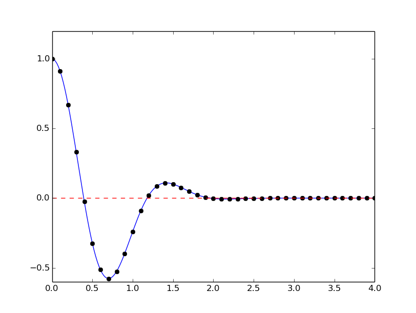
Running this program with some function, say \(f(x)=e^{-x^2}\cos(4x)\) (which has a solution at \(x = \frac{\pi}{8}\)), gives the root 0.392699, which has an error of \(8.2\cdot 10^{-8}\). Increasing the number of points with a factor of ten gives a root with an error of \(3.1\cdot 10^{-10}\).
After such a quick “flat” implementation of an algorithm, we should always try to offer the algorithm as a Matlab function, applicable to as wide a problem domain as possible. The function should take \(f\) and an associated interval \([a,b]\) as input, as well as a number of points (\(n\)), and return a list of all the roots in \([a,b]\). Here is our candidate for a good implementation of the brute force rooting finding algorithm:
function all_roots = brute_force_root_finder(f, a, b, n)
    x = linspace(a, b, n);
    y = f(x);
    roots = [];
    for i = 1:(n-1)
        if y(i)*y(i+1) < 0
            root = x(i) - (x(i+1) - x(i))/(y(i+1) - y(i))*y(i);
            roots = [roots; root];
        end
    end
    all_roots = roots;
end
This function is found in the file brute_force_root_finder.m.
This time we use another elegant technique to indicate if roots were found
or not: roots is empty (an array of length zero) if the root finding was unsuccessful,
otherwise it contains all the roots. Application of the function to
the previous example can be coded as
(demo_brute_force_root_finder.m):
function demo_brute_force_root_finder()
    roots = brute_force_root_finder(
        @(x) exp(-x.^2).*cos(4*x), 0, 4, 1001);
    if length(roots) > 0
        roots
    else
        fprintf('Could not find any roots');
    end
end
Brute force optimization
Numerical algorithm
We realize that \(x_i\) corresponds to a maximum point if \(y_{i-1} < y_i > y_{i+1}\). Similarly, \(x_i\) corresponds to a minimum if \(y_{i-1} > y_i < y_{i+1}\). We can do this test for all “inner” points \(i=1,\ldots,n-1\) to find all local minima and maxima. In addition, we need to add an end point, \(i=0\) or \(i=n\), if the corresponding \(y_i\) is a global maximum or minimum.
Implementation
The algorithm above can be translated to the following Matlab function (file brute_force_optimizer.m):
function [xy_minima, xy_maxima] = brute_force_optimizer(f, a, b, n)
    x = linspace(a, b, n);
    y = f(x);
    % Let maxima and minima hold the indices corresponding
    % to (local) maxima and minima points
    minima = [];
    maxima = [];
    for i = 2:(n-1)
        if y(i-1) < y(i) && y(i) > y(i+1)
            maxima = [maxima; i];
        end
        if y(i-1) > y(i) && y(i) < y(i+1)
            minima = [minima; i];
        end
    end

    % What about the end points?
    y_min_inner = y(minima(1));   % Initialize
    for i = 1:length(minima)
        if y(minima(i)) < y_min_inner
            y_min_inner = y(minima(i));
        end
    end
    y_max_inner = y(maxima(1));   % Initialize
    for i = 1:length(maxima)
        if y(maxima(i)) > y_max_inner
            y_max_inner = y(maxima(i));
        end
    end

    if y(1) > y_max_inner
        maxima = [maxima; 1];
    end
    if y(length(x)) > y_max_inner
       maxima = [maxima; length(x)];
    end
    if y(1) < y_min_inner
        minima = [minima; 1];
    end
    if y(length(x)) < y_min_inner
        minima = [minima; length(x)];
    end

    % Compose return values
    xy_minima = [];
    for i = 1:length(minima)
        xy_minima = [xy_minima; [x(minima(i)) y(minima(i))]];
    end
    xy_maxima = [];
    for i = 1:length(maxima)
        xy_maxima = [xy_maxima; [x(maxima(i)) y(maxima(i))]];
    end
end
An application to \(f(x)=e^{-x^2}\cos(4x)\) looks like
function demo_brute_force_optimizer
    [xy_minima, xy_maxima] = brute_force_optimizer(
        @(x) exp(-x.^2).*cos(4*x), 0, 4, 1001);
    xy_minima
    xy_maxima
end
Model problem for algebraic equations
We shall consider the very simple problem of finding the square root of 9, which is the positive solution of \(x^2=9\). The nice feature of solving an equation whose solution is known beforehand is that we can easily investigate how the numerical method and the implementation perform in the search for the solution. The \(f(x)\) function corresponding to the equation \(x^2=9\) is
Our interval of interest for solutions will be \([0,1000]\) (the upper limit here is chosen somewhat arbitrarily).
In the following, we will present several efficient and accurate methods for solving nonlinear algebraic equations, both single equation and systems of equations. The methods all have in common that they search for approximate solutions. The methods differ, however, in the way they perform the search for solutions. The idea for the search influences the efficiency of the search and the reliability of actually finding a solution. For example, Newton’s method is very fast, but not reliable, while the bisection method is the slowest, but absolutely reliable. No method is best at all problems, so we need different methods for different problems.
What is the difference between linear and nonlinear equations
You know how to solve linear equations \(ax+b=0\): \(x=-b/a\). All other types of equations \(f(x)=0\), i.e., when \(f(x)\) is not a linear function of \(x\), are called nonlinear. A typical way of recognizing a nonlinear equation is to observe that \(x\) is “not alone” as in \(ax\), but involved in a product with itself, such as in \(x^3 + 2x^2 -9=0\). We say that \(x^3\) and \(2x^2\) are nonlinear terms. An equation like \(\sin x + e^x\cos x=0\) is also nonlinear although \(x\) is not explicitly multiplied by itself, but the Taylor series of \(\sin x\), \(e^x\), and \(\cos x\) all involve polynomials of \(x\) where \(x\) is multiplied by itself.
Newton’s method
Newton’s method, also known as Newton-Raphson’s method, is a very famous and widely used method for solving nonlinear algebraic equations. Compared to the other methods we will consider, it is generally the fastest one (usually by far). It does not guarantee that an existing solution will be found, however.
A fundamental idea of numerical methods for nonlinear equations is to construct a series of linear equations (since we know how to solve linear equations) and hope that the solutions of these linear equations bring us closer and closer to the solution of the nonlinear equation. The idea will be clearer when we present Newton’s method and the secant method.
Deriving and implementing Newton’s method
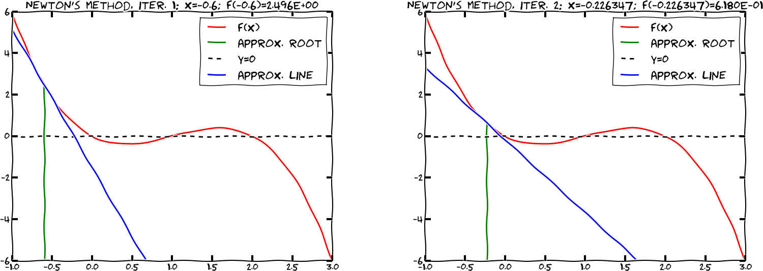
Figure Illustrates the idea of Newton’s method with \( f(x) = x^2 - 9 \) , repeatedly solving for crossing of tangent lines with the \( x \) axis shows the \(f(x)\) function in our model equation \(x^2-9=0\). Numerical methods for algebraic equations require us to guess at a solution first. Here, this guess is called \(x_0\). The fundamental idea of Newton’s method is to approximate the original function \(f(x)\) by a straight line, i.e., a linear function, since it is straightforward to solve linear equations. There are infinitely many choices of how to approximate \(f(x)\) by a straight line. Newton’s method applies the tangent of \(f(x)\) at \(x_0\), see the rightmost tangent in Figure Illustrates the idea of Newton’s method with \( f(x) = x^2 - 9 \) , repeatedly solving for crossing of tangent lines with the \( x \) axis. This linear tangent function crosses the \(x\) axis at a point we call \(x_1\). This is (hopefully) a better approximation to the solution of \(f(x)=0\) than \(x_0\). The next fundamental idea is to repeat this process. We find the tangent of \(f\) at \(x_1\), compute where it crosses the \(x\) axis, at a point called \(x_2\), and repeat the process again. Figure Illustrates the idea of Newton’s method with \( f(x) = x^2 - 9 \) , repeatedly solving for crossing of tangent lines with the \( x \) axis shows that the process brings us closer and closer to the left. It remains, however, to see if we hit \(x=3\) or come sufficiently close to this solution.
Illustrates the idea of Newton’s method with \( f(x) = x^2 - 9 \) , repeatedly solving for crossing of tangent lines with the \( x \) axis
How do we compute the tangent of a function \(f(x)\) at a point \(x_0\)? The tangent function, here called \(\tilde f(x)\), is linear and has two properties:
- the slope equals to \(f'(x_0)\)
- the tangent touches the \(f(x)\) curve at \(x_0\)
So, if we write the tangent function as \(\tilde f(x)=ax+b\), we must require \(\tilde f'(x_0)=f'(x_0)\) and \(\tilde f(x_0)=f(x_0)\), resulting in
The key step in Newton’s method is to find where the tangent crosses the \(x\) axis, which means solving \(\tilde f(x)=0\):
This is our new candidate point, which we call \(x_1\):
With \(x_0 = 1000\), we get \(x_1 \approx 500\), which is in accordance with the graph in Figure Illustrates the idea of Newton’s method with \( f(x) = x^2 - 9 \) , repeatedly solving for crossing of tangent lines with the \( x \) axis. Repeating the process, we get
The general scheme of Newton’s method may be written as
The computation in (162) is repeated until \(f\left(x_n\right)\) is close enough to zero. More precisely, we test if \(|f(x_n)|<\epsilon\), with \(\epsilon\) being a small number.
We moved from 1000 to 250 in two iterations, so it is exciting to see
how fast we can approach the solution \(x=3\).
A computer program can automate the calculations. Our first
try at implementing Newton’s method is in a function naive_Newton:
function result = naive_Newton(f,dfdx,starting_value,eps)
    x = starting_value;
    while abs(f(x)) > eps
        x = x - f(x)/dfdx(x);
    end
    result = x;
end
The argument x is the starting value, called \(x_0\) in our previous
description.
To solve the problem \(x^2=9\) we also need to implement
function result = f(x)
    result = x^2 - 9;
end

function result = dfdx(x)
    result = 2*x;
end
Why not use an array for the \(x\) approximations
Newton’s method is normally formulated with an iteration index \(n\),
Seeing such an index, many would implement this as
x(n+1) = x(x) - f(x(n))/dfdx(x(n));
Such an array is fine, but requires storage of all the approximations.
In large industrial applications, where Newton’s method solves
millions of equations at once, one cannot afford to store all the
intermediate approximations in memory, so then it is important to
understand that the algorithm in Newton’s method has no more need
for \(x_n\) when \(x_{n+1}\) is computed. Therefore, we can work with
one variable x and overwrite the previous value:
x = x - f(x)/dfdx(x)
Running naive_Newton(f, dfdx, 1000, eps=0.001) results in the approximate
solution 3.000027639. A smaller value of eps will produce a more
accurate solution. Unfortunately, the plain naive_Newton function
does not return how many iterations it used, nor does it print out
all the approximations \(x_0,x_1,x_2,\ldots\), which would indeed be a nice
feature. If we insert such a printout, a rerun results in
500.0045
250.011249919
125.02362415
62.5478052723
31.3458476066
15.816483488
8.1927550496
4.64564330569
3.2914711388
3.01290538807
3.00002763928
We clearly see that the iterations approach the solution quickly. This speed of the search for the solution is the primary strength of Newton’s method compared to other methods.
Making a more efficient and robust implementation
The naive_Newton function works fine for the example we are considering
here. However, for more general use, there are some pitfalls that
should be fixed in an improved version of the code. An example
may illustrate what the problem is: let us solve \(\tanh(x)=0\), which
has solution \(x=0\). With \(|x_0|\leq 1.08\) everything works fine. For
example, \(x_0\) leads to six iterations if \(\epsilon=0.001\):
-1.05895313436
0.989404207298
-0.784566773086
0.36399816111
-0.0330146961372
2.3995252668e-05
Adjusting \(x_0\) slightly to 1.09 gives division by zero! The approximations computed by Newton’s method become
-1.09331618202
1.10490354324
-1.14615550788
1.30303261823
-2.06492300238
13.4731428006
-1.26055913647e+11
The division by zero is caused by \(x_7=-1.26055913647\cdot 10^{11}\), because \(\tanh(x_7)\) is 1.0 to machine precision, and then \(f'(x)=1 - \tanh(x)^2\) becomes zero in the denominator in Newton’s method.
The underlying problem, leading to the division by zero in the above
example, is that Newton’s method diverges: the approximations move
further and further away from \(x=0\). If it had not been for the
division by zero, the condition in the while loop would always
be true and the loop would run forever. Divergence of Newton’s method
occasionally happens, and the remedy
is to abort the method when a maximum number of iterations is reached.
Another disadvantage of the naive_Newton function is that it
calls the \(f(x)\) function twice as many times as necessary. This extra
work is of no concern when \(f(x)\) is fast to evaluate, but in
large-scale industrial software, one call to \(f(x)\) might take hours or days, and then removing unnecessary calls is important. The solution
in our function is to store the call f(x) in a variable (f_value)
and reuse the value instead of making a new call f(x).
To summarize, we want to write an improved function for implementing Newton’s method where we
- avoid division by zero
- allow a maximum number of iterations
- avoid the extra evaluation to \(f(x)\)
A more robust and efficient version of the function, inserted in a complete program Newtons_method.m for solving \(x^2 - 9 = 0\), is listed below.
function Newtons_method()
    f = @(x) x^2 - 9;
    dfdx = @(x) 2*x;
    eps = 1e-6;
    x0 = 1000;
    [solution,no_iterations] = Newton(f, dfdx, x0, eps);
    if no_iterations > 0   % Solution found
        fprintf('Number of function calls: %d\n', 1 + 2*no_iterations);
        fprintf('A solution is: %f\n', solution)
    else
        fprintf('Abort execution.\n')
    end
end

function [solution, no_iterations] = Newton(f, dfdx, x0, eps)
    x = x0;
    f_value = f(x);
    iteration_counter = 0;
    while abs(f_value) > eps && iteration_counter < 100
        try
            x = x - (f_value)/dfdx(x);
        catch
            fprintf('Error! - derivative zero for x = \n', x)
            exit(1)
        end
        f_value = f(x);
        iteration_counter = iteration_counter + 1;
    end
    % Here, either a solution is found, or too many iterations
    if abs(f_value) > eps
        iteration_counter = -1;
    end
    solution = x;
    no_iterations = iteration_counter;
end
Handling of the potential division by zero is done by a
try-catch construction, which works as follows. First, Matlab tries to execute the code in the try block, but if something goes wrong there, the catch block is executed instead and the execution is terminated by exit.
The division by zero will always be detected and the program will be stopped. The main purpose of our way of treating the division by zero is to give the user a more informative error message and stop the program in a gentler way.
Calling
exit
with an argument different from zero (here 1)
signifies that the program stopped because of an error.
It is a good habit to supply the value 1, because tools in
the operating system can then be used by other programs to detect
that our program failed.
To prevent an infinite loop because of divergent iterations, we have
introduced the integer variable iteration_counter to count the
number of iterations in Newton’s method.
With iteration_counter we can easily extend the condition in the
while such that no more iterations take place when the number of
iterations reaches 100. We could easily let this limit be an argument
to the function rather than a fixed constant.
The Newton function returns the approximate solution and the number
of iterations. The latter equals \(-1\) if the convergence criterion
\(|f(x)|<\epsilon\) was not reached within the maximum number of
iterations. In the calling code, we print out the solution and
the number of function calls. The main cost of a method for
solving \(f(x)=0\) equations is usually the evaluation of \(f(x)\) and \(f'(x)\),
so the total number of calls to these functions is an interesting
measure of the computational work. Note that in function Newton
there is an initial call to \(f(x)\) and then one call to \(f\) and one
to \(f'\) in each iteration.
Running Newtons_method.m, we get the following printout on the screen:
Number of function calls: 25
A solution is: 3.000000
As we did with the integration methods in the chapter Computing integrals, we will
place our solvers for nonlinear algebraic equations in separate files for easy use by other programs. So, we place Newton in the file Newton.m
The Newton scheme will work better if the starting value is close to the solution. A good starting value may often make the difference as to whether the code actually finds a solution or not. Because of its speed, Newton’s method is often the method of first choice for solving nonlinear algebraic equations, even if the scheme is not guaranteed to work. In cases where the initial guess may be far from the solution, a good strategy is to run a few iterations with the bisection method (see the chapter The bisection method) to narrow down the region where \(f\) is close to zero and then switch to Newton’s method for fast convergence to the solution.
Newton’s method requires the analytical expression for the
derivative \(f'(x)\). Derivation of \(f'(x)\) is not always a reliable
process by hand if \(f(x)\) is a complicated function.
However, Matlab has the Symbolic Math Toolbox, which we may use
to create the required dfdx function (Octave does not (yet) offer
the same possibilities for symbolic computations as Matlab. However,
there is work in progress, e.g. on using SymPy (from Python) from
Octave). In our sample problem, the recipe goes as follows:
syms x;                   % define x as a mathematical symbol
f_expr = x^2 - 9;         % symbolic expression for f(x)
dfdx_expr = diff(f_expr)  % compute f'(x) symbolically
% Turn f_expr and dfdx_expr into plain Matlab functions
f = matlabFunction(f_expr);
dfdx = matlabFunction(dfdx_expr);
dfdx(5)                   % will print 10
The nice feature of this code snippet is that dfdx_expr is the
exact analytical expression for the derivative, 2*x, if you
print it out. This is a symbolic expression so we cannot do
numerical computing with it, but the matlabFunction
turns symbolic expressions into callable Matlab functions.
The next method is the secant method, which is usually slower than Newton’s method, but it does not require an expression for \(f'(x)\), and it has only one function call per iteration.
The secant method
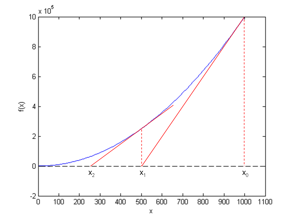
When finding the derivative \(f'(x)\) in Newton’s method is problematic, or when function evaluations take too long; we may adjust the method slightly. Instead of using tangent lines to the graph we may use secants. The approach is referred to as the secant method, and the idea is illustrated graphically in Figure Illustrates the use of secants in the secant method when solving . From two chosen starting values, and the crossing of the corresponding secant with the axis is computed, followed by a similar computation of from and for our example problem \(x^2 - 9 = 0\).
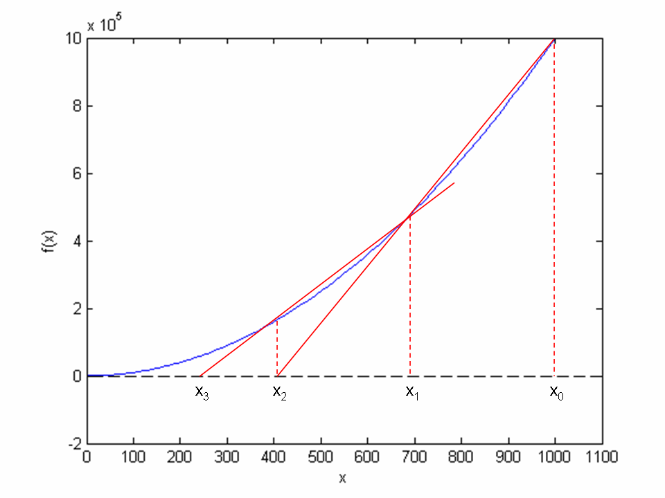
Illustrates the use of secants in the secant method when solving \(x^2 - 9 = 0, x \in [0, 1000]\). From two chosen starting values, \(x_0 = 1000\) and \(x_1 = 700\) the crossing \(x_2\) of the corresponding secant with the \(x\) axis is computed, followed by a similar computation of \(x_3\) from \(x_1\) and \(x_2\)
The idea of the secant method is to think as in Newton’s method, but instead of using \(f'(x_n)\), we approximate this derivative by a finite difference or the secant, i.e., the slope of the straight line that goes through the two most recent approximations \(x_n\) and \(x_{n-1}\). This slope reads
Inserting this expression for \(f'(x_n)\) in Newton’s method simply gives us the secant method:
or
Comparing (164) to the graph in Figure Illustrates the use of secants in the secant method when solving . From two chosen starting values, and the crossing of the corresponding secant with the axis is computed, followed by a similar computation of from and , we see how two chosen starting points (\(x_0 = 1000\), \(x_1= 700\), and corresponding function values) are used to compute \(x_2\). Once we have \(x_2\), we similarly use \(x_1\) and \(x_2\) to compute \(x_3\). As with Newton’s method, the procedure is repeated until \(f(x_n)\) is below some chosen limit value, or some limit on the number of iterations has been reached. We use an iteration counter here too, based on the same thinking as in the implementation of Newton’s method.
We can store the approximations \(x_n\) in an array, but as in Newton’s
method, we notice that the computation of \(x_{n+1}\) only needs
knowledge of \(x_n\) and \(x_{n-1}\), not “older”
approximations. Therefore, we can make use of only three variables:
x for \(x_{n+1}\), x1 for \(x_n\), and x0 for \(x_{n-1}\). Note that
x0 and x1 must be given (guessed) for the algorithm to start.
A program secant_method.m that solves our example problem may be written as:
function secant_method()
    f = @(x) x^2 - 9;
    eps = 1e-6;
    x0 = 1000;  x1 = x0 - 1;
    [solution,no_iterations] = secant(f, x0, x1, eps);
    if no_iterations > 0   % Solution found
        fprintf('Number of function calls: %d\n', 2 + no_iterations);
        fprintf('A solution is: %f\n', solution)
    else
        fprintf('Abort execution.\n')
    end
end

function [solution,no_iterations] = secant(f, x0, x1, eps)
    f_x0 = f(x0);
    f_x1 = f(x1);
    iteration_counter = 0;
    while abs(f_x1) > eps && iteration_counter < 100
        try
            denominator = (f_x1 - f_x0)/(x1 - x0);
            x = x1 - (f_x1)/denominator;
        catch
            fprintf('Error! - denominator zero for x = \n', x1)
            break
        end
        x0 = x1;
        x1 = x;
        f_x0 = f_x1;
        f_x1 = f(x1);
        iteration_counter = iteration_counter + 1;
    end
    % Here, either a solution is found, or too many iterations
    if abs(f_x1) > eps
        iteration_counter = -1;
    end
    solution = x1;
    no_iterations = iteration_counter;
end
The number of function calls is now related to no_iterations,
i.e., the number of iterations, as 2 + no_iterations, since we need
two function calls before entering the while loop, and then one
function call per loop iteration. Note that, even though we need two
points on the graph to compute each updated estimate, only a single
function call (f(x1)) is required in each iteration since
f(x0) becomes the “old” f(x1) and may simply be copied as
f_x0 = f_x1 (the exception is the very first iteration where two function
evaluations are needed).
Running secant_method.m, gives the following printout on the screen:
Number of function calls: 19
A solution is: 3.000000
As with the function Newton, we place secant in
a separate file secant.m for easy use later.
The bisection method
Neither Newton’s method nor the secant method can guarantee that an existing solution will be found (see Exercise 72: Understand why Newton’s method can fail and Exercise 73: See if the secant method fails). The bisection method, however, does that. However, if there are several solutions present, it finds only one of them, just as Newton’s method and the secant method. The bisection method is slower than the other two methods, so reliability comes with a cost of speed.
To solve \(x^2 - 9 = 0\), \(x \in \left[0, 1000\right]\), with the bisection method, we reason as follows. The first key idea is that if \(f(x) = x^2 - 9\) is continuous on the interval and the function values for the interval endpoints (\(x_L = 0\), \(x_R =1000\)) have opposite signs, \(f(x)\) must cross the \(x\) axis at least once on the interval. That is, we know there is at least one solution.
The second key idea comes from dividing the interval in two equal parts, one to the left and one to the right of the midpoint \(x_M = 500\). By evaluating the sign of \(f(x_M)\), we will immediately know whether a solution must exist to the left or right of \(x_M\). This is so, since if \(f(x_M) \ge 0\), we know that \(f(x)\) has to cross the \(x\) axis between \(x_L\) and \(x_M\) at least once (using the same argument as for the original interval). Likewise, if instead \(f(x_M) \le 0\), we know that \(f(x)\) has to cross the \(x\) axis between \(x_M\) and \(x_R\) at least once.
In any case, we may proceed with half the interval only. The exception is if \(f(x_M) \approx 0\), in which case a solution is found. Such interval halving can be continued until a solution is found. A “solution” in this case, is when \(|f(x_M)|\) is sufficiently close to zero, more precisely (as before): \(|f(x_M)|<\epsilon\), where \(\epsilon\) is a small number specified by the user.
The sketched strategy seems reasonable, so let us write a reusable function that can solve a general algebraic equation \(f(x)=0\) (bisection_method.m):
function bisection_method()
    f = @(x) x^2 - 9;
    eps = 1e-6;
    a = 0;   b = 1000;
    [solution, no_iterations] = bisection(f, a, b, eps);
    if solution <= b   % Solution found
        fprintf('Number of function calls: %d\n', 1+2*no_iterations);
        fprintf('A solution is: %f\n', solution);
    else
        fprintf('Abort execution.\n');
    end
end

function [result1, result2] = bisection(f, x_L, x_R, eps)
    if f(x_L)*f(x_R) > 0
        fprintf('Error! Function does not have opposite\n');
        fprintf('signs at interval endpoints!')
        exit(1)
    end
    x_M = (x_L + x_R)/2.0;
    f_M = f(x_M);
    iteration_counter = 1;
    while abs(f_M) > eps
        left_f = f(x_L);
        right_f = f(x_R);
        if left_f*f_M > 0   % i.e., same sign
            x_L = x_M;
        else
            x_R = x_M;
        end
        x_M = (x_L + x_R)/2;
        f_M = f(x_M);
        iteration_counter = iteration_counter + 2;
    end
    result1 = x_M;
    result2 = iteration_counter;
end
Note that we first check if \(f\) changes sign in \([a,b]\), because that is a requirement for the algorithm to work. The algorithm also relies on a continuous \(f(x)\) function, but this is very challenging for a computer code to check.
We get the following printout to the screen when bisection_method.m is run:
Number of function calls: 61
A solution is: 3.000000
We notice that the number of function calls is much higher than with the previous methods.
Required work in the bisection method
If the starting interval of the bisection method is bounded by \(a\) and \(b\), and the solution at step \(n\) is taken to be the middle value, the error is bounded as
As with the two previous methods, the function bisection is
stored as a separate file bisection.m for easy use by other programs.
Rate of convergence
With the methods above, we noticed that the number of iterations or function calls could differ quite substantially. The number of iterations needed to find a solution is closely related to the rate of convergence, which is the speed of the error as we approach the root. More precisely, we introduce the error in iteration \(n\) as \(e_n=|x-x_n|\), and define the convergence rate \(q\) as
where \(C\) is a constant. The exponent \(q\) measures how fast the error is reduced from one iteration to the next. The larger \(q\) is, the faster the error goes to zero, and the fewer iterations we need to meet the stopping criterion \(|f(x)|<\epsilon\).
A single \(q\) in (166) is defined in the limit \(n\rightarrow\infty\). For finite \(n\), and especially smaller \(n\), \(q\) will vary with \(n\). To estimate \(q\), we can compute all the errors \(e_n\) and set up (166) for three consecutive experiments \(n-1\), \(n\), and \(n+1\):
Dividing these two equations by each other and solving with respect to \(q\) gives
Since this \(q\) will vary somewhat with \(n\), we call it \(q_n\). As \(n\) grows, we expect \(q_n\) to approach a limit (\(q_n\rightarrow q\)). To compute all the \(q_n\) values, we need all the \(x_n\) approximations. However, our previous implementations of Newton’s method, the secant method, and the bisection method returned just the final approximation.
Therefore, we have extended those previous implementations such that
the user can choose whether the final value or the whole history of
solutions is to be returned. The extended implementations are named
Newton_solver, secant_solver and bisection_solver. Compared to
the previous implementations, each of these now takes an extra
parameter return_x_list. This parameter is a boolean, set to true
if the function is supposed to return all the root approximations, or
false, if the function should only return the final
approximation. As an example, let us take a closer look at
Newton_solver:
function [sol, no_it] = Newton_solver(f, dfdx, x, eps, return_x_list)
    f_value = f(x);
    iteration_counter = 0;
    if return_x_list
        x_list = [];
    end
    while abs(f_value) > eps && iteration_counter < 100
        try
            x = x - (f_value)/dfdx(x);
        catch
            fprintf('Error! - derivative zero for x = \n', x)
            break
        end
        f_value = f(x);
        iteration_counter = iteration_counter + 1;
        if return_x_list
            x_list = [x_list x];
        end
    end
    % Here, either a solution is found, or too many iterations
    if abs(f_value) > eps
        iteration_counter = -1;   % i.e., lack of convergence
    end

    if return_x_list
        sol = x_list;
        no_it = iteration_counter;
    else
        sol = x;
        no_it = iteration_counter;
    end
end
The function is found in the file Newton_solver.m.
We can now make a call
[x, iter] = Newton_solver(f, dfdx, 1000, 1e-6, true);
and get an array x returned. With knowledge of the exact
solution \(x\) of \(f(x)=0\), we can compute all the errors \(e_n\)
and associated \(q_n\) values with the compact function
function q = rate(x, x_exact)
    e = abs(x - x_exact);
    q = zeros(length(e)-2,1);
    for n = 2:(length(e)-1)
        q(n-1) = log(e(n+1)/e(n))/log(e(n)/e(n-1));
    end
end
The error model (166) works well for Newton’s method and the secant method. For the bisection method, however, it works well in the beginning, but not when the solution is approached.
We can compute the rates \(q_n\) and print them nicely,
function print_rates(method, x, x_exact)
    q = rate(x, x_exact);
    fprintf('%s:\n', method)
    for i = 1:length(q)
        fprintf('%.2f ', q(i));
    end
    fprintf('\n')
end
The result for print_rates('Newton', x, 3) is
Newton:
1.01 1.02 1.03 1.07 1.14 1.27 1.51 1.80 1.97 2.00
indicating that \(q=2\) is the rate for Newton’s method. A similar computation using the secant method, gives the rates
secant:
1.26 0.93 1.05 1.01 1.04 1.05 1.08 1.13 1.20 1.30 1.43
1.54 1.60 1.62 1.62
Here it seems that \(q\approx 1.6\) is the limit.
Remark. If we in the bisection method think of the length of the current interval containing the solution as the error \(e_n\), then (166) works perfectly since \(e_{n+1}=\frac{1}{2}e_n\), i.e., \(q=1\) and \(C=\frac{1}{2}\), but if \(e_n\) is the true error \(|x-x_n|\), it is easily seen from a sketch that this error can oscillate between the current interval length and a potentially very small value as we approach the exact solution. The corresponding rates \(q_n\) fluctuate widely and are of no interest.
Solving multiple nonlinear algebraic equations
So far in this chapter, we have considered a single nonlinear algebraic equation. However, systems of such equations arise in a number of applications, foremost nonlinear ordinary and partial differential equations. Of the previous algorithms, only Newton’s method is suitable for extension to systems of nonlinear equations.
Abstract notation
Suppose we have \(n\) nonlinear equations, written in the following abstract form:
The system can now be written as \(\boldsymbol{F} (\boldsymbol{x}) = \boldsymbol{0}\).
As a specific example on the notation above, the system
can be written in our abstract form by introducing \(x_0=x\) and \(x_1=y\). Then
Taylor expansions for multi-variable functions
We follow the ideas of Newton’s method for one equation in one variable: approximate the nonlinear \(f\) by a linear function and find the root of that function. When \(n\) variables are involved, we need to approximate a vector function \(\boldsymbol{F}(\boldsymbol{x})\) by some linear function \(\tilde\boldsymbol{F} = \boldsymbol{J}\boldsymbol{x} + \boldsymbol{c}\), where \(\boldsymbol{J}\) is an \(n\times n\) matrix and \(\boldsymbol{c}\) is some vector of length \(n\).
The technique for approximating \(\boldsymbol{F}\) by a linear function is to use the first two terms in a Taylor series expansion. Given the value of \(\boldsymbol{F}\) and its partial derivatives with respect to \(\boldsymbol{x}\) at some point \(\boldsymbol{x}_i\), we can approximate the value at some point \(\boldsymbol{x}_{i+1}\) by the two first term in a Taylor series expansion around \(\boldsymbol{x}_i\):
The next terms in the expansions are omitted here and of size \(||\boldsymbol{x}_{i+1}-\boldsymbol{x}_i||^2\), which are assumed to be small compared with the two terms above.
The expression \(\nabla\boldsymbol{F}\) is the matrix of all the partial derivatives of \(\boldsymbol{F}\). Component \((i,j)\) in \(\nabla\boldsymbol{F}\) is
For example, in our \(2\times 2\) system (172)-(173) we can use SymPy to compute the Jacobian:
>>> from sympy import *
>>> x0, x1 = symbols('x0 x1')
>>> F0 = x0**2 - x1 + x0*cos(pi*x0)
>>> F1 = x0*x1 + exp(-x1) - x0**(-1)
>>> diff(F0, x0)
-pi*x0*sin(pi*x0) + 2*x0 + cos(pi*x0)
>>> diff(F0, x1)
-1
>>> diff(F1, x0)
x1 + x0**(-2)
>>> diff(F1, x1)
x0 - exp(-x1)
We can then write
The matrix \(\nabla\boldsymbol{F}\) is called the Jacobian of \(\boldsymbol{F}\) and often denoted by \(\boldsymbol{J}\).
Newton’s method
The idea of Newton’s method is that we have some approximation \(\boldsymbol{x}_i\) to the root and seek a new (and hopefully better) approximation \(\boldsymbol{x}_{i+1}\) by approximating \(\boldsymbol{F}(\boldsymbol{x}_{i+1})\) by a linear function and solve the corresponding linear system of algebraic equations. We approximate the nonlinear problem \(\boldsymbol{F}(\boldsymbol{x}_{i+1})=0\) by the linear problem
where \(\boldsymbol{J}(\boldsymbol{x}_i)\) is just another notation for \(\nabla\boldsymbol{F}(\boldsymbol{x}_i)\). The equation (174) is a linear system with coefficient matrix \(\boldsymbol{J}\) and right-hand side vector \(\boldsymbol{F}(\boldsymbol{x}_i)\). We therefore write this system in the more familiar form
where we have introduce a symbol \(\boldsymbol{\delta}\) for the unknown vector \(\boldsymbol{x}_{i+1}-\boldsymbol{x}_i\) that multiplies the Jacobian \(\boldsymbol{J}\).
The \(i\)-th iteration of Newton’s method for systems of algebraic equations consists of two steps:
- Solve the linear system \(\boldsymbol{J}(\boldsymbol{x}_i)\boldsymbol{\delta} = -\boldsymbol{F}(\boldsymbol{x}_i)\) with respect to \(\boldsymbol{\delta}\).
- Set \(\boldsymbol{x}_{i+1} = \boldsymbol{x}_i + \boldsymbol{\delta}\).
Solving systems of linear equations must make use of appropriate
software. Gaussian elimination is the most common, and in general
the most robust, method for this purpose.
Matlab interfaces the well-known LAPACK package with
high-quality and very well tested subroutines for linear algebra.
The backslash operator solves a linear system \(Ax=b\) by x = A\b
by a method based on Gaussian elimination.
When nonlinear systems of algebraic equations arise from discretization of partial differential equations, the Jacobian is very often sparse, i.e., most of its elements are zero. In such cases it is important to use algorithms that can take advantage of the many zeros. Gaussian elimination is then a slow method, and (much) faster methods are based on iterative techniques.
Implementation
Here is a very simple implementation of Newton’s method for systems of nonlinear algebraic equations:
% Use Newton's method to solve systems of nonlinear algebraic equations.

function [x, iteration_counter] = Newton_system(F, J, x, eps)
    % Solve nonlinear system F=0 by Newton's method.
    % J is the Jacobian of F. Both F and J must be functions of x.
    % At input, x holds the start value. The iteration continues
    % until ||F|| < eps.

    F_value = F(x);
    F_norm = norm(F_value);  % l2 norm of vector
    iteration_counter = 0;
    while abs(F_norm) > eps && iteration_counter < 100
        delta = J(x)\-F_value;
        x = x + delta;
        F_value = F(x);
        F_norm = norm(F_value);
        iteration_counter = iteration_counter + 1;
    end

    % Here, either a solution is found, or too many iterations
    if abs(F_norm) > eps
        iteration_counter = -1;
    end

end
We can test the function Newton_system with the
\(2\times 2\) system (172)-(173):
function test_Newton_system1()
    expected = [1; 0];
    tol = 1e-4;
    [x, n] = Newton_system(@F, @J, [2; -1], 0.0001);
    error = abs(expected - x);
    assert(norm(error) < tol, 'err=%g', error);
end

function F_vector = F(x)
    F_vector = [x(1)^2 - x(2) + x(1)*cos(pi*x(1));...
                x(1)*x(2) + exp(-x(2)) - x(1)^(-1)];
end

function J_matrix = J(x)
    J_matrix = [2*x(1) + cos(pi*x(1)) - pi*x(1)*sin(pi*x(1)) -1;...
                x(2) + x(1)^(-2) x(1) - exp(-x(2))];
end
Here, the testing is based on the L2 norm of the error vector. Alternatively, we could test against the
values of x that the algorithm finds, with appropriate tolerances.
For example, as chosen for the error norm, if eps=0.0001, a tolerance of \(10^{-4}\) can be used for
x[0] and x[1].
Exercises
Exercise 72: Understand why Newton’s method can fail
The purpose of this exercise is to understand when Newton’s method works and fails. To this end, solve \(\tanh x=0\) by Newton’s method and study the intermediate details of the algorithm. Start with \(x_0=1.08\). Plot the tangent in each iteration of Newton’s method. Then repeat the calculations and the plotting when \(x_0=1.09\). Explain what you observe.
Solution. The program may be written as:
function [solution, no_iterations] =...
                                Newton_failure(f, dfdx, x0, eps)
    x = x0;
    f_value = f(x);
    iteration_counter = 0;
    while abs(f_value) > eps && iteration_counter < 100
        try
            fprintf('Current x vaule: %g \n', x);
            plot_line(f, x, f_value, dfdx(x));
            x = x - (f_value)/dfdx(x);
        catch
            fprintf('Error! - derivative zero for x = \n', x)
            exit(1)
        end
        f_value = f(x);
        iteration_counter = iteration_counter + 1;
    end
    % Here, either a solution is found, or too many iterations
    if abs(f_value) > eps
        iteration_counter = -1;
    end
    solution = x;
    no_iterations = iteration_counter;
end
which may be called from the script use_my_Newton_failure.m:
f = @(x) tanh(x);
dfdx = @(x) 1 - tanh(x)^2;

[solution, no_iterations] = Newton_failure(f, dfdx, 1.08, 0.001)

if no_iterations > 0      % Solution found
    fprintf('Number of function calls: %d \n', 1 + 2*no_iterations);
    fprintf('A solution is: %f \n', solution);
else
    fprintf('Solution not found! \n');
end
Note that Newton_failure.m calls the function plot_line (located in plot_line.m),
reading:
function plot_line(f, xn, f_xn, slope)
    % Plot both f(x) and the tangent or secant
    x_f = linspace(-2, 2, 100);
    y_f = f(x_f);
    x_t = linspace(xn-2, xn+2, 10);
    y_t = slope*x_t + (f_xn - slope*xn); % Straight line: ax + b
    figure();
    plot(x_t, y_t, 'r-', x_f, y_f, 'b-');   grid('on');
    xlabel('x'); ylabel('f(x)');
    disp('...press enter to continue')
    pause on; pause;
end
(The function plot_line is placed as a separate m-file so that it may be used also
by the function secant_failure, which is to be written in another exercise.)
Running the program with x set to \(1.08\) produces a series of plots (and prints) showing
the graph and the tangent for the present value of x. There are quite many
plots, so we do not show them here. However, the tangent line “jumps” around
a few times before it settles. In the final plot the tangent line goes through
the solution at \(x = 0\). The final printout brings the information:
Number of function calls: 13
A solution is: 0.000024
When we run the program anew, this time with x set to \(1.09\), we get another series of
plots (and prints), but this time the tangent moves away from the (known) solution.
The final printout we get states that:
Number of function calls: 19
A solution is: nan
Here, nan stands for “not a number”, meaning that we got no solution value for x.
That is, Newton’s method diverged.
Filename: Newton_failure.*.
Exercise 73: See if the secant method fails
Does the secant method behave better than Newton’s method in the problem described in Exercise 72: Understand why Newton’s method can fail? Try the initial guesses
- \(x_0=1.08\) and \(x_1=1.09\)
- \(x_0=1.09\) and \(x_1=1.1\)
- \(x_0=1\) and \(x_1=2.3\)
- \(x_0=1\) and \(x_1=2.4\)
Solution. The program may be written as:
% This file is not yet written.
which may be called from the script use_my_secant_failure.m:
f = @(x) tanh(x);
dfdx = @(x) 1 - tanh(x)^2;

% Requested trials:
%x0 = 1.08 , x1 = 1.09
%x0 = 1.09 , x1 = 1.1
%x0 = 1 , x1 = 2.3
%x0 = 1 , x1 = 2.4
[solution, no_iterations] = Secant_failure(f, 1, 2.4, 0.001)

if no_iterations > 0       % Solution found
    fprintf('Number of function calls: %d \n', 1 + 2*no_iterations);
    fprintf('A solution is: %f \n', solution);
else
    fprintf('Solution not found! \n');
end
Note that, as with Newton_failure.m, the script plot_line.m is called for
plotting each tangent.
The script converges with the three first-mentioned alternatives for \(x_0\) and \(x_1\). With the final set of parameter values, the method diverges with a printout:
Error! - denominator zero for x = 360.600893792
and a few more lines stating that an exception error has occurred.
Filename: secant_failure.*.
Exercise 74: Understand why the bisection method cannot fail
Solve the same problem as in Exercise 72: Understand why Newton’s method can fail, using the bisection method, but let the initial interval be \([-5,3]\). Report how the interval containing the solution evolves during the iterations.
Solution. The code may be written as:
function [result1, result2] = ...
                           bisection_nonfailure(f, x_L, x_R, eps)
    if f(x_L)*f(x_R) > 0
       fprintf('Error! Function does not have opposite \n');
       fprintf('signs at interval endpoints!');
       exit(1);
    end
    x_M = (x_L + x_R)/2;
    f_M = f(x_M);
    iteration_counter = 1;
    while abs(f_M) > eps
        left_f = f(x_L);
        right_f = f(x_R);
        if left_f*f_M > 0            % i.e., same sign
            x_L = x_M;
        else
            x_R = x_M;
        end
        fprintf('interval: [%f, %f]\n', x_L, x_R);
        x_M = (x_L + x_R)/2;
        f_M = f(x_M);
        iteration_counter = iteration_counter + 1;
    end
    result1 = x_M;
    result2 = iteration_counter;
end
which may be called from the script use_my_bisection_nonfailure.m:
f = @(x) tanh(x);

a = -5; b = 3;

[solution, no_iterations] =...
                   bisection_nonfailure(f, a, b, 1.0e-6);

fprintf('Number of function calls: %d\n',1 + 2*no_iterations);
fprintf('A solution is: %f\n', solution);
Running the program produces the following printout:
interval: [-1.000000, 3.000000]
interval: [-1.000000, 1.000000]
Number of function calls: 7
A solution is: 0.000000
Filename: bisection_nonfailure.*.
Exercise 75: Combine the bisection method with Newton’s method
An attractive idea is to combine the reliability of the bisection method with the speed of Newton’s method. Such a combination is implemented by running the bisection method until we have a narrow interval, and then switch to Newton’s method for speed.
Write a function that implements this idea. Start with an interval \([a,b]\) and switch to Newton’s method when the current interval in the bisection method is a fraction \(s\) of the initial interval (i.e., when the interval has length \(s(b-a)\)). Potential divergence of Newton’s method is still an issue, so if the approximate root jumps out of the narrowed interval (where the solution is known to lie), one can switch back to the bisection method. The value of \(s\) must be given as an argument to the function, but it may have a default value of 0.1.
Try the new method on \(\tanh(x)=0\) with an initial interval \([-10,15]\).
Solution. The code may be written as:
function [solution, no_iterations] = ...
                      bisection_Newton(f, dfdx, x_L, x_R, eps, s)
    f_L = f(x_L);
    if f_L*f(x_R) > 0
        fprintf('Error! Function does not have opposite');
        fprintf('signs at interval endpoints!');
        exit(1);
    end
    x_M = (x_L + x_R)/2;
    f_M = f(x_M);
    iteration_counter = 1;
    interval_Newton = s*(x_R - x_L);  % Limit for swith to Newton
    while (x_R - x_L) > interval_Newton
        if f_L*f_M > 0    % i.e., same sign
            x_L = x_M;
            f_L = f_M;
        else
            x_R = x_M;
        end
        x_M = (x_L + x_R)/2;
        f_M = f(x_M);
        iteration_counter = iteration_counter + 1;
    end
    [x, no_iter] = Newton(f, dfdx, x_M, eps);
    solution = x;
    no_iterations = iteration_counter + no_iter;
end
which may be called from the script use_my_bisection_Newton.m:
f = @(x) tanh(x);
dfdx = @(x) 1 - tanh(x)^2;

eps = 1e-6;
a = -10; b = 15;
s = 0.1;
[solution, no_iterations] =...
                        bisection_Newton(f, dfdx, a, b, eps, s);
fprintf('A solution x = %f was reached in %d iterations \n',...
                                       solution, no_iterations);
Running the program produces the following printout:
A solution x = 0.000000 was reached in 7 iterations
Filename: bisection_Newton.m.
Exercise 76: Write a test function for Newton’s method
The purpose of this function is to verify the implementation of Newton’s
method in the Newton function in the file
Newton.m
Construct an algebraic equation and perform two iterations of Newton’s
method by
hand.
Find the corresponding size of \(|f(x)|\) and use this
as value for eps when calling Newton. The function should then
also perform two iterations and return the same approximation to
the root as you calculated manually. Implement this idea for a unit test
as a test function test_Newton().
Solution. Here is the complete module with the test function.
function test_Newton()
    f = @(x) cos(x) + sin(x);
    dfdx = @(x) cos(x) - sin(x);
    x0 = 2;                     % initial guess
    %% Run two iterations with Newton's method
    x1 = x0 - f(x0)/dfdx(x0);
    x2 = x1 - f(x1)/dfdx(x1);
    x_expected = zeros(2,1);
    x_expected(1) = x1;  x_expected(2) = x2;
    eps = f(x_expected(length(x_expected)));  % this eps gives two iterations

    [x_computed, it_counter] = Newton_solver(f, dfdx, x0, eps, true);
    assert(it_counter == 2);
    tol = 1E-15;
    assert(abs(x_computed(1) - x_expected(1)) < tol);
    assert(abs(x_computed(2) - x_expected(2)) < tol);
end
Filename: test_Newton.m.
Exercise 77: Solve nonlinear equation for a vibrating beam
An important engineering problem that arises in a lot of applications is the vibrations of a clamped beam where the other end is free. This problem can be analyzed analytically, but the calculations boil down to solving the following nonlinear algebraic equation:
where \(\beta\) is related to important beam parameters through
where \(\varrho\) is the density of the beam, \(A\) is the area of the cross section, \(E\) is Young’s modulus, and \(I\) is the moment of the inertia of the cross section. The most important parameter of interest is \(\omega\), which is the frequency of the beam. We want to compute the frequencies of a vibrating steel beam with a rectangular cross section having width \(b=25\) mm and height \(h=8\) mm. The density of steel is \(7850 \mbox{ kg/m}^3\), and \(E= 2\cdot 10^{11}\) Pa. The moment of inertia of a rectangular cross section is \(I=bh^3/12\).
a) Plot the equation to be solved so that one can inspect where the zero crossings occur.
Hint. When writing the equation as \(f(\beta)=0\), the \(f\) function increases its amplitude dramatically with \(\beta\). It is therefore wise to look at an equation with damped amplitude, \(g(\beta) = e^{-\beta}f(\beta) = 0\). Plot \(g\) instead.
Solution.
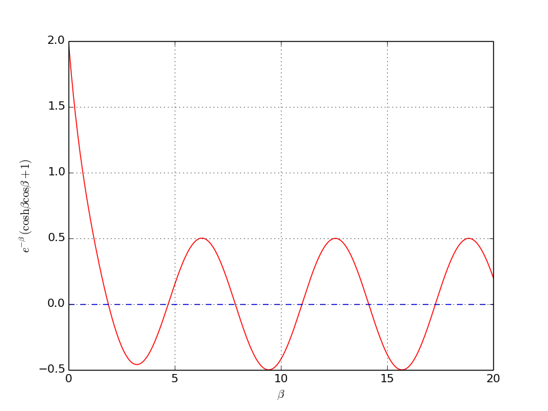
b) Compute the first three frequencies.
Solution. Here is a complete program, using the Bisection method for root finding, based on intervals found from the plot above.
function beam_vib()

    plot_f()

    f_handle = @f;
    % Set up suitable intervals
    intervals = [1 3; 4 6; 7 9];
    betas = [];  % roots
    for i = 1:length(intervals)
        beta_L = intervals(i, 1);  beta_R = intervals(i, 2);
        [beta, it] = bisection(f_handle, beta_L, beta_R, eps=1E-6);
        betas = [betas beta];
        f(beta)
    end
    betas

    % Find corresponding frequencies

    function value = omega(beta, rho, A, E, I)
        value = sqrt(beta^4/(rho*A/(E*I)));
    end

    rho = 7850;  % kg/m^3
    E = 1.0E+11; % Pa
    b = 0.025;   % m
    h = 0.008;   % m
    A = b*h;
    I = b*h^3/12;

    for i = 1:length(betas)
        omega(betas(i), rho, A, E, I)
    end

end

function value = f(beta)
    value = cosh(beta).*cos(beta) + 1;
end

function value = damped(beta)
    % Damp the amplitude of f. It grows like cosh, i.e. exp.
    value = exp(-beta).*f(beta);
end

function plot_f()
    beta = linspace(0, 20, 501);
    %y = f(x)
    y = damped(beta);
    plot(beta, y, 'r', [beta(1), beta(length(beta))], [1, 1], 'b--')
    grid('on');
    xlabel('beta');
    ylabel('exp(-beta) (cosh(beta) cos(beta) +1)')
    savefig('tmp1.png'); savefig('tmp1.pdf')
end
The output of \(\beta\) reads \(1.875\), \(4.494\), \(7.855\), and corresponding \(\omega\) values are \(29\), \(182\), and \(509\) Hz.
Filename: beam_vib.m.
