Solving ordinary differential equations

Differential equations constitute one of the most powerful mathematical tools to understand and predict the behavior of dynamical systems in nature, engineering, and society. A dynamical system is some system with some state, usually expressed by a set of variables, that evolves in time. For example, an oscillating pendulum, the spreading of a disease, and the weather are examples of dynamical systems. We can use basic laws of physics, or plain intuition, to express mathematical rules that govern the evolution of the system in time. These rules take the form of differential equations. You are probably well experienced with equations, at least equations like \(ax+b=0\) or \(ax^2 + bx + c=0\). Such equations are known as algebraic equations, and the unknown is a number. The unknown in a differential equation is a function, and a differential equation will almost always involve this function and one or more derivatives of the function. For example, \(f'(x)=f(x)\) is a simple differential equation (asking if there is any function \(f\) such that it equals its derivative - you might remember that \(e^x\) is a candidate).

The present chapter starts with explaining how easy it is to solve both single (scalar) first-order ordinary differential equations and systems of first-order differential equations by the Forward Euler method. We demonstrate all the mathematical and programming details through two specific applications: population growth and spreading of diseases.

Then we turn to a physical application: oscillating mechanical systems, which arise in a wide range of engineering situations. The differential equation is now of second order, and the Forward Euler method does not perform well. This observation motivates the need for other solution methods, and we derive the Euler-Cromer scheme [1], the 2nd- and 4th-order Runge-Kutta schemes, as well as a finite difference scheme (the latter to handle the second-order differential equation directly without reformulating it as a first-order system). The presentation starts with undamped free oscillations and then treats general oscillatory systems with possibly nonlinear damping, nonlinear spring forces, and arbitrary external excitation. Besides developing programs from scratch, we also demonstrate how to access ready-made implementations of more advanced differential equation solvers in Matlab.

[1]	The term scheme is used as synonym for method or computational recipe, especially in the context of numerical methods for differential equations.

As we progress with more advanced methods, we develop more sophisticated and reusable programs, and in particular, we incorporate good testing strategies so that we bring solid evidence to correct computations. Consequently, the beginning with population growth and disease modeling examples has a very gentle learning curve, while that curve gets significantly steeper towards the end of the treatment of differential equations for oscillatory systems.

Population growth

Our first taste of differential equations regards modeling the growth of some population, such as a cell culture, an animal population, or a human population. The ideas even extend trivially to growth of money in a bank. Let \(N(t)\) be the number of individuals in the population at time \(t\). How can we predict the evolution of \(N(t)\) in time? Below we shall derive a differential equation whose solution is \(N(t)\). The equation reads

\[\tag{29} N'(t) = rN(t),\]

where \(r\) is a number. Note that although \(N\) is an integer in real life, we model \(N\) as a real-valued function. We are forced to do this because the solution of differential equations are (normally continuous) real-valued functions. An integer-valued \(N(t)\) in the model would lead to a lot of mathematical difficulties.

With a bit of guessing, you may realize that \(N(t)=Ce^{rt}\), where \(C\) is any number. To make this solution unique, we need to fix \(C\), done by prescribing the value of \(N\) at some time, usually \(t=0\). Say \(N(0)\) is given as \(N_0\). Then \(N(t)=N_0e^{rt}\).

In general, a differential equation model consists of a differential equation, such as (29) and an initial condition, such as \(N(0)=N_0\). With a known initial condition, the differential equation can be solved for the unknown function and the solution is unique.

It is, of course, very seldom that we can find the solution of a differential equation as easy as in this example. Normally, one has to apply certain mathematical methods, but these can only handle some of the simplest differential equations. However, we can easily deal with almost any differential equation by applying numerical methods and a bit of programming. This is exactly the topic of the present chapter.

Derivation of the model

It can be instructive to show how an equation like (29) arises. Consider some population of (say) an animal species and let \(N(t)\) be the number of individuals in a certain spatial region, e.g. an island. We are not concerned with the spatial distribution of the animals, just the number of them in some spatial area where there is no exchange of individuals with other spatial areas. During a time interval \(\Delta t\), some animals will die and some new will be born. The number of deaths and births are expected to be proportional to \(N\). For example, if there are twice as many individuals, we expect them to get twice as many newborns. In a time interval \(\Delta t\), the net growth of the population will be

\[N(t+\Delta t) - N(t) = \bar b N(t) - \bar d N(t),\]

where \(\bar bN(t)\) is the number of newborns and \(\bar d N(t)\) is the number of deaths. If we double \(\Delta t\), we expect the proportionality constants \(\bar b\) and \(\bar d\) to double too, so it makes sense to think of \(\bar b\) and \(\bar d\) as proportional to \(\Delta t\) and “factor out” \(\Delta t\). That is, we introduce \(b=\bar b/\Delta t\) and \(d=\bar d/\Delta t\) to be proportionality constants for newborns and deaths independent of \(\Delta t\). Also, we introduce \(r=b-d\), which is the net rate of growth of the population per time unit. Our model then becomes

\[\tag{30} N(t+\Delta t) - N(t) = \Delta t\, r N(t)\thinspace .\]

Equation (30) is actually a computational model. Given \(N(t)\), we can advance the population size by

\[N(t+\Delta t) = N(t) + \Delta t\, rN(t)\thinspace .\]

This is called a difference equation. If we know \(N(t)\) for some \(t\), e.g., \(N(0)=N_0\), we can compute

\[\begin{split}N(\Delta t) &= N_0 + \Delta t\, rN_0,\\ N(2\Delta t) &= N(\Delta t) + \Delta t\, rN(\Delta t),\\ N(3\Delta t) &= N(2\Delta t) + \Delta t\, rN(2\Delta t),\\ & \vdots\\ N((k+1)\Delta t) &= N(k\Delta t) + \Delta t\, rN(k\Delta t),\end{split}\]

where \(k\) is some arbitrary integer. A computer program can easily compute \(N((k+1)\Delta t)\) for us with the aid of a little loop.

Warning

Observe that the computational formula cannot be started unless we have an initial condition!

The solution of \(N'=rN\) is \(N=Ce^{rt}\) for any constant \(C\), and the initial condition is needed to fix \(C\) so the solution becomes unique. However, from a mathematical point of view, knowing \(N(t)\) at any point \(t\) is sufficient as initial condition. Numerically, we more literally need an initial condition: we need to know a starting value at the left end of the interval in order to get the computational formula going.

In fact, we do not need a computer since we see a repetitive pattern when doing hand calculations, which leads us to a mathematical formula for \(N((k+1)\Delta t)\), :

\[\begin{split}N((k+1)\Delta t) &= N(k\Delta t) + \Delta t\, rN(k\Delta t) = N(k\Delta t)(1+\Delta t\, r)\\ &= N((k-1)\Delta t)(1+\Delta t\,r)^2\\ &\vdots\\ &= N_0(1+\Delta t\,r)^{k+1}\thinspace .\end{split}\]

Rather than using (30) as a computational model directly, there is a strong tradition for deriving a differential equation from this difference equation. The idea is to consider a very small time interval \(\Delta t\) and look at the instantaneous growth as this time interval is shrunk to an infinitesimally small size. In mathematical terms, it means that we let \(\Delta t\rightarrow 0\). As (30) stands, letting \(\Delta t\rightarrow 0\) will just produce an equation \(0=0\), so we have to divide by \(\Delta t\) and then take the limit:

\[\lim_{\Delta t\rightarrow 0}\frac{N(t+\Delta t)-N(t)}{\Delta t} = rN(t)\thinspace .\]

The term on the left-hand side is actually the definition of the derivative \(N'(t)\), so we have

\[N'(t) = rN(t),\]

which is the corresponding differential equation.

There is nothing in our derivation that forces the parameter \(r\) to be constant - it can change with time due to, e.g., seasonal changes or more permanent environmental changes.

Detour: Exact mathematical solution

If you have taken a course on mathematical solution methods for differential equations, you may want to recap how an equation like \(N'=rN\) or \(N'=r(t)N\) is solved. The method of separation of variables is the most convenient solution strategy in this case:

\[\begin{split}N' &=rN\\ \frac{dN}{dt} &= rN\\ \frac{dN}{N} &= rdt\\ \int_{N_0}^N \frac{dN}{N} &= \int_0^t rdt\\ \ln N - \ln N_0 &= \int_0^t r(t)dt\\ N &= N_0\exp{(\int_0^t r(t)dt)},\end{split}\]

which for constant \(r\) results in \(N=N_0e^{rt}\). Note that \(\exp{(t)}\) is the same as \(e^t\).

As will be described later, \(r\) must in more realistic models depend on \(N\). The method of separation of variables then requires to integrate \(\int_{N_0}^{N} N/r(N)dN\), which quickly becomes non-trivial for many choices of \(r(N)\). The only generally applicable solution approach is therefore a numerical method.

Numerical solution

There is a huge collection of numerical methods for problems like (30), and in general any equation of the form \(u'=f(u,t)\), where \(u(t)\) is the unknown function in the problem, and \(f\) is some known formula of \(u\) and optionally \(t\). For example, \(f(u,t)=ru\) in (30). We will first present a simple finite difference method solving \(u'=f(u,t)\). The idea is four-fold:

1. Introduce a mesh in time with \(N_t+1\) points \(t_0,t_1,\ldots,t_{N_t}\). We seek the unknown \(u\) at the mesh points \(t_n\), and introduce \(u^n\) as the numerical approximation to \(u(t_n)\), see Figure Mesh in time with corresponding discrete values (unknowns).
2. Assume that the differential equation is valid at the mesh points.
3. Approximate derivatives by finite differences, see Figure Illustration of a forward difference approximation to the derivative.
4. Formulate a computational algorithm that can compute a new value \(u^n\) based on previously computed values \(u^i\), \(i<n\).

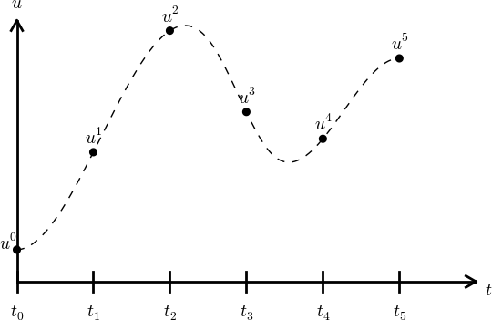
Mesh in time with corresponding discrete values (unknowns)

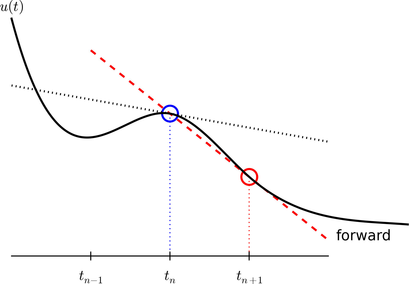
Illustration of a forward difference approximation to the derivative

An example will illustrate the steps. First, we introduce the mesh, and very often the mesh is uniform, meaning that the spacing between points \(t_n\) and \(t_{n+1}\) is constant. This property implies that

\[t_n = n\Delta t,\quad n=0,1,\ldots, N_t\thinspace .\]

Second, the differential equation is supposed to hold at the mesh points. Note that this is an approximation, because the differential equation is originally valid at all real values of \(t\). We can express this property mathematically as

\[u'(t_n)=f(u^n,t_n),\quad n=0,1,\ldots,N_t\thinspace .\]

For example, with our model equation \(u'=ru\), we have the special case

\[u'(t_n)=ru^n,\quad n=0,1,\ldots,N_t,\]

or

\[u'(t_n)=r(t_n)u^n,\quad n=0,1,\ldots,N_t,\]

if \(r\) depends explicitly on \(t\).

Third, derivatives are to be replaced by finite differences. To this end, we need to know specific formulas for how derivatives can be approximated by finite differences. One simple possibility is to use the definition of the derivative from any calculus book,

\[u'(t) = \lim_{\Delta t\rightarrow 0}\frac{u(t+\Delta t)-u(t)}{\Delta t}\thinspace .\]

At an arbitrary mesh point \(t_n\) this definition can be written as

\[u'(t_n) = \lim_{\Delta t\rightarrow 0}\frac{u^{n+1}-u^n}{\Delta t}\thinspace .\]

Instead of going to the limit \(\Delta t\rightarrow 0\) we can use a small \(\Delta t\), which yields a computable approximation to \(u'(t_n)\):

\[u'(t_n) \approx \frac{u^{n+1}-u^n}{\Delta t}\thinspace .\]

This is known as a forward difference since we go forward in time (\(u^{n+1}\)) to collect information in \(u\) to estimate the derivative. Figure Illustration of a forward difference approximation to the derivative illustrates the idea. The error in of the forward difference is proportional to \(\Delta t\) (often written as \({\mathcal{O}(\Delta t)}\), but will not use this notation in the present book).

We can now plug in the forward difference in our differential equation sampled at the arbitrary mesh point \(t_n\):

\[\tag{31} \frac{u^{n+1}-u^n}{\Delta t} = f(u^n,t_n),\]

or with \(f(u,t)=ru\) in our special model problem for population growth,

\[\tag{32} \frac{u^{n+1}-u^n}{\Delta t} = ru^n\thinspace .\]

If \(r\) depends on time, we insert \(r(t_n)=r^n\) for \(r\) in this latter equation.

The fourth step is to derive a computational algorithm. Looking at (31), we realize that if \(u^n\) should be known, we can easily solve with respect to \(u^{n+1}\) to get a formula for \(u\) at the next time level \(t_{n+1}\):

\[\tag{33} u^{n+1}= u^n + \Delta t f(u^n,t_n)\thinspace .\]

Provided we have a known starting value, \(u^0=U_0\), we can use (33) to advance the solution by first computing \(u^1\) from \(u^0\), then \(u^2\) from \(u^1\), \(u^3\) from \(u^2\), and so forth.

Such an algorithm is called a numerical scheme for the differential equation and often written compactly as

\[\tag{34} u^{n+1}= u^n + \Delta t f(u^n,t_n),\quad u^0=U_0,\quad n=0,1,\ldots,N_t-1\thinspace .\]

This scheme is known as the Forward Euler scheme, also called Euler’s method.

In our special population growth model, we have

\[\tag{35} u^{n+1}= u^n + \Delta t\, ru^n,\quad u^0=U_0,\quad n=0,1,\ldots,N_t-1\thinspace .\]

We may also write this model using the problem-specific symbol \(N\) instead of the generic \(u\) function:

\[\tag{36} N^{n+1}= N^n + \Delta t\, rN^n,\quad N^0=N_0,\quad n=0,1,\ldots,N_t-1\thinspace .\]

The observant reader will realize that (36) is nothing but the computational model (30) arising directly in the model derivation. The formula (36) arises, however, from a detour via a differential equation and a numerical method for the differential equation. This looks rather unnecessary! The reason why we bother to derive the differential equation model and then discretize it by a numerical method is simply that the discretization can be done in many ways, and we can create (much) more accurate and more computationally efficient methods than (36) or (34). This can be useful in many problems! Nevertheless, the Forward Euler scheme is intuitive and widely applicable, at least when \(\Delta t\) is chosen to be small.

The numerical solution between the mesh points

Our numerical method computes the unknown function \(u\) at discrete mesh points \(t_1,t_2,\ldots,t_{N_t}\). What if we want to evaluate the numerical solution between the mesh points? The most natural choice is to assume a linear variation between the mesh points, see Figure The numerical solution at points can be extended by linear segments between the mesh points. This is compatible with the fact that when we plot the array \(u^0,u^1,\ldots\) versus \(t_0,t_1,\ldots\), a straight line is drawn between the discrete points.

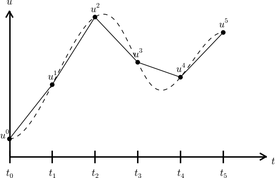
The numerical solution at points can be extended by linear segments between the mesh points

Programming the Forward Euler scheme; the special case

Let us compute (36) in a program. The input variables are \(N_0\), \(\Delta t\), \(r\), and \(N_t\). Note that we need to compute \(N_t+1\) new values \(N^1,\ldots,N^{N_t+1}\). A total of \(N_t+2\) values are needed in an array representation of \(N^n\), \(n=0,\ldots,N_t+1\).

Our first version of this program is as simple as possible:

N_0 = input('Give initial population size N_0: ');
r   = input('Give net growth rate r: ');
dt  = input('Give time step size: ');
N_t = input('Give number of steps: ');
t = linspace(0, (N_t+1)*dt, N_t+2);
N = zeros(N_t+2, 1);

N(1) = N_0;
for n = 1:N_t
    N(n+1) = N(n) + r*dt*N(n);
end

if N_t < 70
    numerical_sol = 'bo';
else
    numerical_sol = 'b-';
end
plot(t, N, numerical_sol, t, N_0*exp(r.*t), 'r-');
xlabel('t'); ylabel('N(t)');
legend('numerical', 'exact', 'location', 'northwest');
filestem = strcat('growth1_', num2str(N_t), 'steps');
print(filestem, '-dpng');  print(filestem, '-dpdf');

The complete code above resides in the file growth1.m.

Let us demonstrate a simulation where we start with 100 animals, a net growth rate of 10 percent (0.1) per time unit, which can be one month, and \(t\in [0,20]\) months. We may first try \(\Delta t\) of half a month (0.5), which implies \(N_t=40\) (or to be absolutely precise, the last time point to be computed according to our set-up above is \(t_{N_t+1}=20.5\)). Figure Evolution of a population computed with time step 0.5 month shows the results. The solid line is the exact solution, while the circles are the computed numerical solution. The discrepancy is clearly visible. What if we make \(\Delta t\) 10 times smaller? The result is displayed in Figure Evolution of a population computed with time step 0.05 month, where we now use a solid line also for the numerical solution (otherwise, 400 circles would look very cluttered, so the program has a test on how to display the numerical solution, either as circles or a solid line). We can hardly distinguish the exact and the numerical solution. The computing time is also a fraction of a second on a laptop, so it appears that the Forward Euler method is sufficiently accurate for practical purposes. (This is not always true for large, complicated simulation models in engineering, so more sophisticated methods may be needed.)

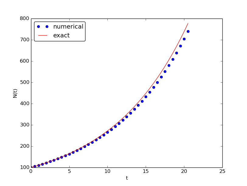
Evolution of a population computed with time step 0.5 month

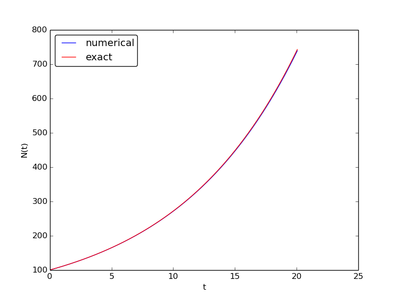
Evolution of a population computed with time step 0.05 month

It is also of interest to see what happens if we increase \(\Delta t\) to 2 months. The results in Figure Evolution of a population computed with time step 2 months indicate that this is an inaccurate computation.

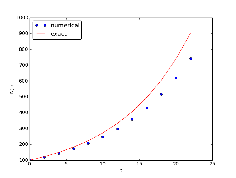
Evolution of a population computed with time step 2 months

Understanding the Forward Euler method

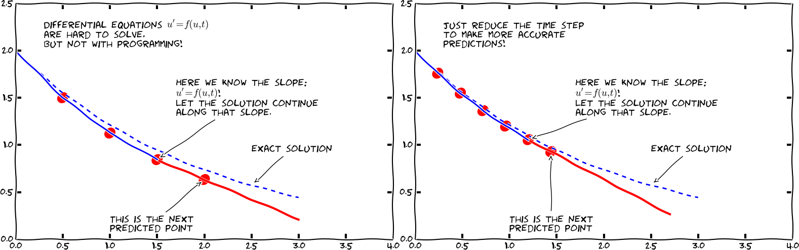
The good thing about the Forward Euler method is that it gives an understanding of what a differential equation is and a geometrical picture of how to construct the solution. The first idea is that we have already computed the solution up to some time point \(t_n\). The second idea is that we want to progress the solution from \(t_n\) to \(t_{n+1}\) as a straight line.

We know that the line must go through the solution at \(t_n\), i.e., the point \((t_n, u^n)\). The differential equation tells us the slope of the line: \(u'(t_n) = f(u^n,t_n)=ru^n\). That is, the differential equation gives a direct formula for the further direction of the solution curve. We can say that the differential equation expresses how the system (\(u\)) undergoes changes at a point.

There is a general formula for a straight line \(y=ax+b\) with slope \(a\) that goes through the point \((x_0,y_0)\): \(y=a(x-x_0)+y_0\). Using this formula adapted to the present case, and evaluating the formula for \(t_{n+1}\), results in

\[u^{n+1} = ru^n(t_{n+1} - t_n) + u^n = u^n + \Delta t\,ru^n,\]

which is nothing but the Forward Euler formula. You are now encouraged to do Exercise 43: Geometric construction of the Forward Euler method to become more familiar with the geometric interpretation of the Forward Euler method.

Programming the Forward Euler scheme; the general case

Our previous program was just a flat main program tailored to a special differential equation. When programming mathematics, it is always good to consider a (large) class of problems and making a Matlab function to solve any problem that fits into the class. More specifically, we will make software for the class of differential equation problems of the form

\[u'(t)=f(u,t),\quad u=U_0,\ t\in [0,T],\]

for some given function \(f\), and numbers \(U_0\) and \(T\). We also take the opportunity to illustrate what is commonly called a demo function. As the name implies, the purpose of such a function is solely to demonstrate how the function works (not to be confused with a test function, which does verification by use of assert). The Matlab function calculating the solution must take \(f\), \(U_0\), \(\Delta t\), and \(T\) as input, find the corresponding \(N_t\), compute the solution, and return and array with \(u^0,u^1,\ldots,u^{N_t}\) and an array with \(t_0,t_1,\ldots,t_{N_t}\). The Forward Euler scheme reads

\[u^{n+1}=u^n + \Delta t f(u^n,t_n),\quad n=0,\ldots,N_t-1\thinspace .\]

The corresponding program ode_FE.m may now take the form

function [sol, time] = ode_FE(f, U_0, dt, T)
    N_t = floor(T/dt);
    u = zeros(N_t+1, 1);
    t = linspace(0, N_t*dt, length(u));
    u(1) = U_0;
    for n = 1:N_t
        u(n+1) = u(n) + dt*f(u(n), t(n));
    end
    sol  = u;
    time = t;
end

Note that the function ode_FE is general, i.e. it can solve any differential equation \(u'=f(u,t)\).

A proper demo function for this solver might be written as (file demo_population_growth.m):

function demo_population_growth()
    % Test case: u' = r*u, u(0)=100
    function r = f(u, t)
        r = 0.1*u;
    end
    [u, t] = ode_FE(@f, 100, 0.5, 20);
    plot(t, u, t, 100*exp(0.1*t));
end

The solution should be identical to what the growth1.m program produces with the same parameter settings (\(r=0.1\), \(N_0=100\)). This feature can easily be tested by inserting a print statement, but a much better, automated verification is suggested in Exercise 43: Geometric construction of the Forward Euler method. You are strongly encouraged to take a “break” and do that exercise now.

Remark on the use of u as variable

In the ode_FE program, the variable u is used in different contexts. Inside the ode_FE function, u is an array, but in the f(u,t) function, as exemplified in the demo_population_growth function, the argument u is a number. Typically, we call f (in ode_FE) with the u argument as one element of the array u in the ode_FE function: u(n).

Making the population growth model more realistic

Exponential growth of a population according the model \(N'=rN\), with exponential solution \(N=N_0e^{rt}\), is unrealistic in the long run because the resources needed to feed the population are finite. At some point there will not be enough resources and the growth will decline. A common model taking this effect into account assumes that \(r\) depends on the size of the population, \(N\):

\[N(t+\Delta t) - N(t) = r(N(t))N(t)\thinspace .\]

The corresponding differential equation becomes

\[N' = r(N)N\thinspace .\]

The reader is strongly encouraged to repeat the steps in the derivation of the Forward Euler scheme and establish that we get

\[N^{n+1} = N^n + \Delta t\, r(N^n)N^n,\]

which computes as easy as for a constant \(r\), since \(r(N^n)\) is known when computing \(N^{n+1}\). Alternatively, one can use the Forward Euler formula for the general problem \(u'=f(u,t)\) and use \(f(u,t)=r(u)u\) and replace \(u\) by \(N\).

The simplest choice of \(r(N)\) is a linear function, starting with some growth value \(\bar r\) and declining until the population has reached its maximum, \(M\), according to the available resources:

\[r(N) = \bar r(1 - N/M)\thinspace .\]

In the beginning, \(N\ll M\) and we will have exponential growth \(e^{\bar rt}\), but as \(N\) increases, \(r(N)\) decreases, and when \(N\) reaches \(M\), \(r(N)=0\) so there is now more growth and the population remains at \(N(t)=M\). This linear choice of \(r(N)\) gives rise to a model that is called the logistic model. The parameter \(M\) is known as the carrying capacity of the population.

Let us run the logistic model with aid of the ode_FE function in the ode_FE module. We choose \(N(0)=100\), \(\Delta t=0.5\) month, \(T=60\) months, \(r=0.1\), and \(M=500\). The complete program, called logistic.m, is basically a call to ode_FE:

f = @(u, t) 0.1*(1 - u/500)*u;
U_0 = 100;

dt = 0.5;  T = 60;
[u, t] = ode_FE(f, U_0, dt, T);
plot(t, u, 'b-');
xlabel('t');  ylabel('N(t)');
filestem = strcat('tmp_',num2str(dt));
% Note: this print statement gets a problem with the decimal point
%print(filestem,'-dpng');  print(filestem,'-dpdf');
% so we rather do it like this:
filename = strcat(filestem, '.png'); print(filename);
filename = strcat(filestem, '.pdf'); print(filename);

dt = 20;  T = 100;
[u, t] = ode_FE(f, U_0, dt, T);
plot(t, u, 'b-');
xlabel('t');  ylabel('N(t)');
filestem = strcat('tmp_',num2str(dt));
print(filestem, '-dpng');  print(filestem, '-dpdf');

Figure Logistic growth of a population shows the resulting curve. We see that the population stabilizes around \(M=500\) individuals. A corresponding exponential growth would reach \(N_0e^{rt}=100e^{0.1\cdot 60}\approx 40,300\) individuals!

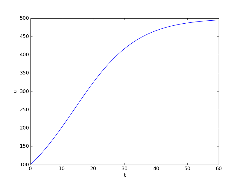
Logistic growth of a population

It is always interesting to see what happens with large \(\Delta t\) values. We may set \(\Delta t=20\) and \(T=100\). Now the solution, seen in Figure Logistic growth with large time step, oscillates and is hence qualitatively wrong, because one can prove that the exact solution of the differential equation is monotone. (However, there is a corresponding difference equation model, \(N_{n+1}=rN_n(1-N_n/M)\), which allows oscillatory solutions and those are observed in animal populations. The problem with large \(\Delta t\) is that it just leads to wrong mathematics - and two wrongs don’t make a right in terms of a relevant model.)

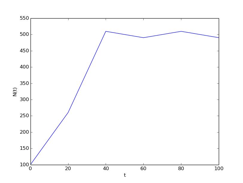
Logistic growth with large time step

Remark on the world population

The number of people on the planet follows the model \(N'=r(t)N\), where the net reproduction \(r(t)\) varies with time and has decreased since its top in 1990. The current world value of \(r\) is 1.2%, and it is difficult to predict future values. At the moment, the predictions of the world population point to a growth to 9.6 billion before declining.

This example shows the limitation of a differential equation model: we need to know all input parameters, including \(r(t)\), in order to predict the future. It is seldom the case that we know all input parameters. Sometimes knowledge of the solution from measurements can help estimate missing input parameters.

Verification: exact linear solution of the discrete equations

How can we verify that the programming of an ODE model is correct? The best method is to find a problem where there are no unknown numerical approximation errors, because we can then compare the exact solution of the problem with the result produced by our implementation and expect the difference to be within a very small tolerance. We shall base a unit test on this idea and implement a corresponding test function (see the section Constructing unit tests and writing test functions) for automatic verification of our implementation.

It appears that most numerical methods for ODEs will exactly reproduce a solution \(u\) that is linear in \(t\). We may therefore set \(u=at+b\) and choose any \(f\) whose derivative is \(a\). The choice \(f(u,t)=a\) is very simple, but we may add anything that is zero, e.g.,

\[f(u,t) = a + (u - (at+b))^m.\]

This is a valid \(f(u,t)\) for any \(a\), \(b\), and \(m\). The corresponding ODE looks highly non-trivial, however:

\[u' = a + (u - (at+b))^m.\]

Using the general ode_FE function in ode_FE.m, we may write a proper test function as follows (in file test_ode_FE_exact_linear.m):

function test_ode_FE_exact_linear()
    % Test if a linear function u(t) = a*x + b is exactly reproduced.

    a = 4;  b = -1;  m = 6;

    exact_solution = @(t) (a*t + b)';
    f = @(u, t) a + (u - exact_solution(t))^m;

    dt = 0.5;       T = 20.0;

    [u, t] = ode_FE(f, exact_solution(0), dt, T);
    diff = max(abs(exact_solution(t) - u));
    tol = 1E-15;           % Tolerance for float comparison
    assert(diff < tol);
end

Observe that we cannot compare diff to zero, which is what we mathematically expect, because diff is a floating-point variable that most likely contains small rounding errors. Therefore, we must compare diff to zero with a tolerance, here \(10^{-15}\).

You are encouraged to do Exercise 44: Make test functions for the Forward Euler method where the goal is to make a test function for a verification based on comparison with hand-calculated results for a few time steps.

Spreading of diseases

Our aim with this section is to show in detail how one can apply mathematics and programming to investigate spreading of diseases. The mathematical model is now a system of three differential equations with three unknown functions. To derive such a model, we can use mainly intuition, so no specific background knowledge of diseases is required.

Spreading of a flu

Imagine a boarding school out in the country side. This school is a small and closed society. Suddenly, one or more of the pupils get a flu. We expect that the flu may spread quite effectively or die out. The question is how many of the pupils and the school’s staff will be affected. Some quite simple mathematics can help us to achieve insight into the dynamics of how the disease spreads.

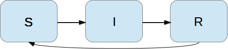
Let the mathematical function \(S(t)\) count how many individuals, at time \(t\), that have the possibility to get infected. Here, \(t\) may count hours or days, for instance. These individuals make up a category called susceptibles, labeled as S. Another category, I, consists of the individuals that are infected. Let \(I(t)\) count how many there are in category I at time \(t\). An individual having recovered from the disease is assumed to gain immunity. There is also a small possibility that an infected will die. In either case, the individual is moved from the I category to a category we call the removed category, labeled with R. We let \(R(t)\) count the number of individuals in the \(R\) category at time \(t\). Those who enter the \(R\) category, cannot leave this category.

To summarize, the spreading of this disease is essentially the dynamics of moving individuals from the S to the I and then to the R category:

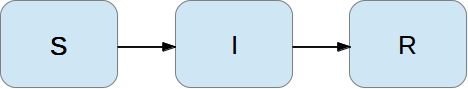
We can use mathematics to more precisely describe the exchange between the categories. The fundamental idea is to describe the changes that take place during a small time interval, denoted by \(\Delta t\).

Our disease model is often referred to as a compartment model, where quantities are shuffled between compartments (here a synonym for categories) according to some rules. The rules express changes in a small time interval \(\Delta t\), and from these changes we can let \(\Delta t\) go to zero and obtain derivatives. The resulting equations then go from difference equations (with finite \(\Delta t\)) to differential equations (\(\Delta t\rightarrow 0\)).

We introduce a uniform mesh in time, \(t_n=n\Delta t\), \(n=0,\ldots,N_t\), and seek \(S\) at the mesh points. The numerical approximation to \(S\) at time \(t_n\) is denoted by \(S^n\). Similarly, we seek the unknown values of \(I(t)\) and \(R(t)\) at the mesh points and introduce a similar notation \(I^n\) and \(R^n\) for the approximations to the exact values \(I(t_n)\) and \(R(t_n)\).

In the time interval \(\Delta t\) we know that some people will be infected, so \(S\) will decrease. We shall soon argue by mathematics that there will be \(\beta\Delta tSI\) new infected individuals in this time interval, where \(\beta\) is a parameter reflecting how easy people get infected during a time interval of unit length. If the loss in \(S\) is \(\beta\Delta tSI\), we have that the change in \(S\) is

\[\tag{37} S^{n+1} - S^n = -\beta\Delta tS^nI^n\thinspace .\]

Dividing by \(\Delta t\) and letting \(\Delta t\rightarrow 0\), makes the left-hand side approach \(S'(t_n)\) such that we obtain a differential equation

\[\tag{38} S' = -\beta SI\thinspace .\]

The reasoning in going from the difference equation (37) to the differential equation (38) follows exactly the steps explained in the section Derivation of the model.

Before proceeding with how \(I\) and \(R\) develops in time, let us explain the formula \(\beta\Delta tSI\). We have \(S\) susceptibles and \(I\) infected people. These can make up \(SI\) pairs. Now, suppose that during a time interval \(T\) we measure that \(m\) actual pairwise meetings do occur among \(n\) theoretically possible pairings of people from the S and I categories. The probability that people meet in pairs during a time \(T\) is (by the empirical frequency definition of probability) equal to \(m/n\), i.e., the number of successes divided by the number of possible outcomes. From such statistics we normally derive quantities expressed per unit time, i.e., here we want the probability per unit time, \(\mu\), which is found from dividing by \(T\): \(\mu = m/(nT)\).

Given the probability \(\mu\), the expected number of meetings per time interval of \(SI\) possible pairs of people is (from basic statistics) \(\mu SI\). During a time interval \(\Delta t\), there will be \(\mu SI\Delta t\) expected number of meetings between susceptibles and infected people such that the virus may spread. Only a fraction of the \(\mu\Delta t SI\) meetings are effective in the sense that the susceptible actually becomes infected. Counting that \(m\) people get infected in \(n\) such pairwise meetings (say 5 are infected from 1000 meetings), we can estimate the probability of being infected as \(p=m/n\). The expected number of individuals in the S category that in a time interval \(\Delta t\) catch the virus and get infected is then \(p\mu\Delta t SI\). Introducing a new constant \(\beta =p\mu\) to save some writing, we arrive at the formula \(\beta\Delta tSI\).

The value of \(\beta\) must be known in order to predict the future with the disease model. One possibility is to estimate \(p\) and \(\mu\) from their meanings in the derivation above. Alternatively, we can observe an “experiment” where there are \(S_0\) susceptibles and \(I_0\) infected at some point in time. During a time interval \(T\) we count that \(N\) susceptibles have become infected. Using (37) as a rough approximation of how \(S\) has developed during time \(T\) (and now \(T\) is not necessarily small, but we use (37) anyway), we get

\[\tag{39} N = \beta T S_0I_0\quad\Rightarrow\quad\beta = {N\over TS_0I_0}\thinspace .\]

We need an additional equation to describe the evolution of \(I(t)\). Such an equation is easy to establish by noting that the loss in the S category is a corresponding gain in the I category. More precisely,

\[\tag{40} I^{n+1} - I^n = \beta\Delta tS^nI^n\thinspace .\]

However, there is also a loss in the I category because people recover from the disease. Suppose that we can measure that \(m\) out of \(n\) individuals recover in a time period \(T\) (say 10 of 40 sick people recover during a day: \(m=10\), \(n=40\), \(T=24\) h). Now, \(\gamma =m/(nT)\) is the probability that one individual recovers in a unit time interval. Then (on average) \(\gamma\Delta t I\) infected will recover in a time interval \(\Delta t\). This quantity represents a loss in the I category and a gain in the R category. We can therefore write the total change in the I category as

\[\tag{41} I^{n+1} - I^n = \beta\Delta tS^nI^n - \gamma\Delta t I^n\thinspace .\]

The change in the R category is simple: there is always an increase from the I category:

\[\tag{42} R^{n+1} - R^n = \gamma\Delta t I^n\thinspace .\]

Since there is no loss in the R category (people are either recovered and immune, or dead), we are done with the modeling of this category. In fact, we do not strictly need the equation (42) for \(R\), but extensions of the model later will need an equation for \(R\).

Dividing by \(\Delta t\) in (41) and (42) and letting \(\Delta t\rightarrow 0\), results in the corresponding differential equations

\[\tag{43} I' = \beta\Delta tSI - \gamma\Delta t I,\]

and

\[\tag{44} R' = \gamma I\thinspace .\]

To summarize, we have derived difference equations (37)-(42), and alternative differential equations (43)-(44). For reference, we list the complete set of the three difference equations:

\[\tag{45} S^{n+1} = S^n -\beta\Delta tS^nI^n,\]

\[\tag{46} I^{n+1} = I^n + \beta\Delta tS^nI^n - \gamma\Delta t I^n,\]

\[\tag{47} R^{n+1} = R^n + \gamma\Delta t I^n\thinspace .\]

Note that we have isolated the new unknown quantities \(S^{n+1}\), \(I^{n+1}\), and \(R^{n+1}\) on the left-hand side, such that these can readily be computed if \(S^n\), \(I^n\), and \(R^n\) are known. To get such a procedure started, we need to know \(S^0\), \(I^0\), \(R^0\). Obviously, we also need to have values for the parameters \(\beta\) and \(\gamma\).

We also list the system of three differential equations:

\[\tag{48} S' = -\beta SI,\]

\[\tag{49} I' = \beta SI - \gamma I,\]

\[\tag{50} R' = \gamma I\thinspace .\]

This differential equation model (and also its discrete counterpart above) is known as a SIR model. The input data to the differential equation model consist of the parameters \(\beta\) and \(\gamma\) as well as the initial conditions \(S(0)=S_0\), \(I(0)=I_0\), and \(R(0)=R_0\).

A Forward Euler method for the differential equation system

Let us apply the same principles as we did in the section Numerical solution to discretize the differential equation system by the Forward Euler method. We already have a time mesh and time-discrete quantities \(S^n\), \(I^n\), \(R^n\), \(n=0,\ldots,N_t\). The three differential equations are assumed to be valid at the mesh points. At the point \(t_n\) we then have

\[\tag{51} S'(t_n) = -\beta S(t_n)I(t_n),\]

\[\tag{52} I'(t_n) = \beta S(t_n)I(t_n) - \gamma I(t_n),\]

\[\tag{53} R'(t_n) = \gamma I(t_n),\]

for \(n=0,1,\ldots,N_t\). This is an approximation since the differential equations are originally valid at all times \(t\) (usually in some finite interval \([0,T]\)). Using forward finite differences for the derivatives results in an additional approximation,

\[\tag{54} \frac{S^{n+1}- S^n}{\Delta t} = -\beta S^nI^n,\]

\[\tag{55} \frac{I^{n+1}- I^n}{\Delta t} = \beta S^nI^n - \gamma I^n,\]

\[\tag{56} \frac{R^{n+1}- R^n}{\Delta t} = \gamma I^n\thinspace .\]

As we see, these equations are identical to the difference equations that naturally arise in the derivation of the model. However, other numerical methods than the Forward Euler scheme will result in slightly different difference equations.

Programming the numerical method; the special case

The computation of (54)-(56) can be readily made in a computer program SIR1.m:

% Time unit: 1 h
beta = 10/(40*8*24);
gamma = 3/(15*24);
dt = 0.1;               % 6 min
D = 30;                 % Simulate for D days
N_t = floor(D*24/dt);   % Corresponding no of hours

t = linspace(0, N_t*dt, N_t+1);
S = zeros(N_t+1, 1);
I = zeros(N_t+1, 1);
R = zeros(N_t+1, 1);

% Initial condition
S(1) = 50;
I(1) = 1;
R(1) = 0;

% Step equations forward in time
for n = 1:N_t
   S(n+1) = S(n) - dt*beta*S(n)*I(n);
   I(n+1) = I(n) + dt*beta*S(n)*I(n) - dt*gamma*I(n);
   R(n+1) = R(n) + dt*gamma*I(n);
end

plot(t, S, t, I, t, R);
legend('S', 'I', 'R', 'Location','northwest');
xlabel('hours');
print('tmp', '-dpdf');  print('tmp', '-dpng');

This program was written to investigate the spreading of a flu at the mentioned boarding school, and the reasoning for the specific choices \(\beta\) and \(\gamma\) goes as follows. At some other school where the disease has already spread, it was observed that in the beginning of a day there were 40 susceptibles and 8 infected, while the numbers were 30 and 18, respectively, 24 hours later. Using 1 h as time unit, we then have from (39) that \(\beta = 10/(40\cdot 8\cdot 24)\). Among 15 infected, it was observed that 3 recovered during a day, giving \(\gamma = 3/(15\cdot 24)\). Applying these parameters to a new case where there is one infected initially and 50 susceptibles, gives the graphs in Figure Natural evolution of a flu at a boarding school. These graphs are just straight lines between the values at times \(t_i=i\Delta t\) as computed by the program. We observe that \(S\) reduces as \(I\) and \(R\) grows. After about 30 days everyone has become ill and recovered again.

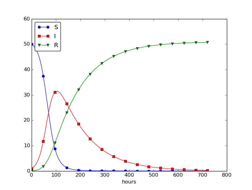
Natural evolution of a flu at a boarding school

We can experiment with \(\beta\) and \(\gamma\) to see whether we get an outbreak of the disease or not. Imagine that a “wash your hands” campaign was successful and that the other school in this case experienced a reduction of \(\beta\) by a factor of 5. With this lower \(\beta\) the disease spreads very slowly so we simulate for 60 days. The curves appear in Figure Small outbreak of a flu at a boarding school ( \( beta \) is much smaller than in Figure :ref:`sec:de:flu:fig1`).

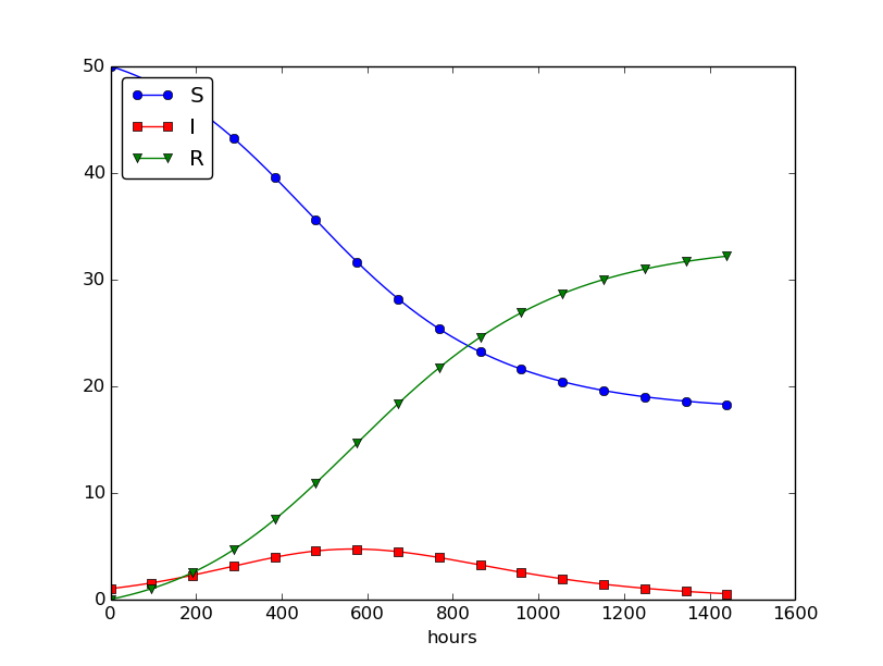
Small outbreak of a flu at a boarding school ( \( beta \) is much smaller than in Figure :ref:`sec:de:flu:fig1`)

Outbreak or not

Looking at the equation for \(I\), it is clear that we must have \(\beta SI - \gamma I>0\) for \(I\) to increase. When we start the simulation it means that

\[\begin{split}\beta S(0)I(0) - \gamma I(0)>0,\end{split}\]

or simpler

\[\begin{split}\tag{57} \frac{\beta S(0)}{\gamma} > 1\end{split}\]

to increase the number of infected people and accelerate the spreading of the disease. You can run the SIR1.m program with a smaller \(\beta\) such that (57) is violated and observe that there is no outbreak.

The power of mathematical modeling

The reader should notice our careful use of words in the previous paragraphs. We started out with modeling a very specific case, namely the spreading of a flu among pupils and staff at a boarding school. With purpose we exchanged words like pupils and flu with more neutral and general words like individuals and disease, respectively. Phrased equivalently, we raised the abstraction level by moving from a specific case (flu at a boarding school) to a more general case (disease in a closed society). Very often, when developing mathematical models, we start with a specific example and see, through the modeling, that what is going on of essence in this example also will take place in many similar problem settings. We try to incorporate this generalization in the model so that the model has a much wider application area than what we aimed at in the beginning. This is the very power of mathematical modeling: by solving one specific case we have often developed more generic tools that can readily be applied to solve seemingly different problems. The next sections will give substance to this assertion.

Abstract problem and notation

When we had a specific differential equation with one unknown, we quickly turned to an abstract differential equation written in the generic form \(u'=f(u,t)\). We refer to such a problem as a scalar ODE. A specific equation corresponds to a specific choice of the formula \(f(u,t)\) involving \(u\) and (optionally) \(t\).

It is advantageous to also write a system of differential equations in the same abstract notation,

\[u'=f(u,t),\]

but this time it is understood that \(u\) is a vector of functions and \(f\) is also vector. We say that \(u'=f(u,t)\) is a vector ODE or system of ODEs in this case. For the SIR model we introduce the two 3-vectors, one for the unknowns,

\[u = (S(t), I(t), R(t)),\]

and one for the right-hand side functions,

\[f(u,t) = (-\beta SI, \beta SI -\gamma I, \gamma I)\thinspace .\]

The equation \(u'=f(u,t)\) means setting the two vectors equal, i.e., each component must be equal. Since \(u'=(S', I', R')\), we get that \(u'=f\) implies

\[\begin{split}S' &= -\beta SI,\\ I' &= \beta SI - \gamma I,\\ R' &= \gamma I\thinspace .\end{split}\]

The generalized short notation \(u'=f(u,t)\) is very handy since we can derive numerical methods and implement software for this abstract system and in a particular application just identify the formulas in the \(f\) vector, implement these, and call functionality that solves the differential equation system.

Programming the numerical method; the general case

In Matlab code, the Forward Euler step

\[u^{n+1} = u^n + \Delta t f(u^n, t_n),\]

being a scalar or a vector equation, can be coded as

u(n+1,:) = u(n,:) + dt*f(u(n,:), t(n))

both in the scalar and vector case. In the vector case, u(n,:) is a one-dimensional array of length \(m+1\) holding the mathematical quantity \(u^n\), and the Matlab function f must return an array of length \(m+1\). Then the expression u(n,:) + dt*f(u(n,:), t(n)) is an array plus a scalar times an array.

For all this to work, the complete numerical solution must be represented by a two-dimensional array, created by u = zeros(N_t+1, m+1). The first index counts the time points and the second the components of the solution vector at one time point. That is, u(n,i) corresponds to the mathematical quantity \(u^n_i\). Writing u(n,:) picks out all the components in the solution at the time point with index n. The nice feature of these facts is that the same piece of Matlab code works for both a scalar ODE and a system of ODEs!

The ode_FE function for the vector ODE is placed in the file ode_system_FE.m and was written as follows:

function [u, t] = ode_FE(f, U_0, dt, T)
    N_t = floor(T/dt);
    u = zeros(N_t+1, length(U_0));
    t = linspace(0, N_t*dt, length(u));
    u(1,:) = U_0;      % Initial values
    t(1) = 0;
    for n = 1:N_t
        u(n+1,:)  = u(n,:) + dt*f(u(n,:), t(n));
    end
end

Let us show how the previous SIR model can be solved using the new general ode_FE that can solve any vector ODE. The user’s f(u, t) function takes a vector u, with three components corresponding to \(S\), \(I\), and \(R\) as argument, along with the current time point t(n), and must return the values of the formulas of the right-hand sides in the vector ODE. An appropriate implementation is

function result = f(u, t)
    S = u(1); I = u(2); R = u(3);
    result = [-beta*S*I beta*S*I - gamma*I gamma*I]
end

where beta and gamma are problem specific parameters set outside of that function. Note that the S, I, and R values correspond to \(S^n\), \(I^n\), and \(R^n\). These values are then just inserted in the various formulas in the vector ODE.

We can now show a function (in file demo_SIR.m) that runs the previous SIR example, but which applies the generic ode_FE function:

function demo_SIR()
    % Test case using an SIR model

    dt = 0.1;               % 6 min
    D = 30;                 % Simulate for D days
    N_t = floor(D*24/dt);   % Corresponding no of hours
    T = dt*N_t;             % End time
    U_0 = [50 1 0];

    f_handle = @f;

    [u, t] = ode_FE(f_handle, U_0, dt, T);

    S = u(:,1);
    I = u(:,2);
    R = u(:,3);
    plot(t, S, 'b-', t, I, 'r-', t, R, 'g-');
    legend('S', 'I', 'R');
    xlabel('hours');
    % Consistency check:
    N = S(1) + I(1) + R(1);
    eps = 1E-12;           % Tolerance for comparing real numbers
    for n = 1:length(S)
        err = abs(S(n) + I(n) + R(n) - N);
        if (err > eps)
            error('demo_SIR: error=%g', err);
        end
    end
end

function result = f(u,t)
    beta = 10/(40*8*24);
    gamma = 3/(15*24);

    S = u(1); I = u(2); R = u(3);
    result = [-beta*S*I beta*S*I - gamma*I gamma*I];
end

Recall that the u returned from ode_FE contains all components (\(S\), \(I\), \(R\)) in the solution vector at all time points. We therefore need to extract the \(S\), \(I\), and \(R\) values in separate arrays for further analysis and easy plotting.

Another key feature of this higher-quality code is the consistency check. By adding the three differential equations in the SIR model, we realize that \(S' + I' + R'=0\), which means that \(S+I+R=\mbox{const}\). We can check that this relation holds by comparing \(S^n+I^n+R^n\) to the sum of the initial conditions. The check is not a full-fledged verification, but it is a much better than doing nothing and hoping that the computation is correct. Exercise 47: Find an appropriate time step; SIR model suggests another method for controlling the quality of the numerical solution.

Time-restricted immunity

Let us now assume that immunity after the disease only lasts for some certain time period. This means that there is transport from the R state to the S state:

Modeling the loss of immunity is very similar to modeling recovery from the disease: the amount of people losing immunity is proportional to the amount of recovered patients and the length of the time interval \(\Delta t\). We can therefore write the loss in the R category as \(-\nu\Delta t R\) in time \(\Delta t\), where \(\nu^{-1}\) is the typical time it takes to lose immunity. The loss in \(R(t)\) is a gain in \(S(t)\). The “budgets” for the categories therefore become

\[\tag{58} S^{n+1} = S^n -\beta\Delta tS^nI^n + \nu\Delta t R^n,\]

\[\tag{59} I^{n+1} = I^n + \beta\Delta tS^nI^n - \gamma\Delta t I^n,\]

\[\tag{60} R^{n+1} = R^n + \gamma\Delta t I^n - \nu\Delta t R^n\thinspace .\]

Dividing by \(\Delta t\) and letting \(\Delta t\rightarrow 0\) gives the differential equation system

\[\tag{61} S' = -\beta SI + \nu R,\]

\[\tag{62} I' = \beta SI - \gamma I,\]

\[\tag{63} R' = \gamma I - \nu R\thinspace .\]

This system can be solved by the same methods as we demonstrated for the original SIR model. Only one modification in the program is necessary: adding nu*R[n] to the S[n+1] update and subtracting the same quantity in the R[n+1] update:

for n = 1:N_t
    S(n+1) = S(n) - dt*beta*S(n)*I(n) + dt*nu*R(n)
    I(n+1) = I(n) + dt*beta*S(n)*I(n) - dt*gamma*I(n)
    R(n+1) = R(n) + dt*gamma*I(n) - dt*nu*R(n)
end

The modified code is found in the file SIR2.m.

Setting \(\nu^{-1}\) to 50 days, reducing \(\beta\) by a factor of 4 compared to the previous example (\(\beta=0.00033\)), and simulating for 300 days gives an oscillatory behavior in the categories, as depicted in Figure Including loss of immunity. It is easy now to play around and study how the parameters affect the spreading of the disease. For example, making the disease slightly more effective (increase \(\beta\) to 0.00043) and increasing the average time to loss of immunity to 90 days lead to other oscillations in Figure Increasing \( beta \) and reducing \( nu \) compared to Figure :ref:`sec:de:flu:fig3`.

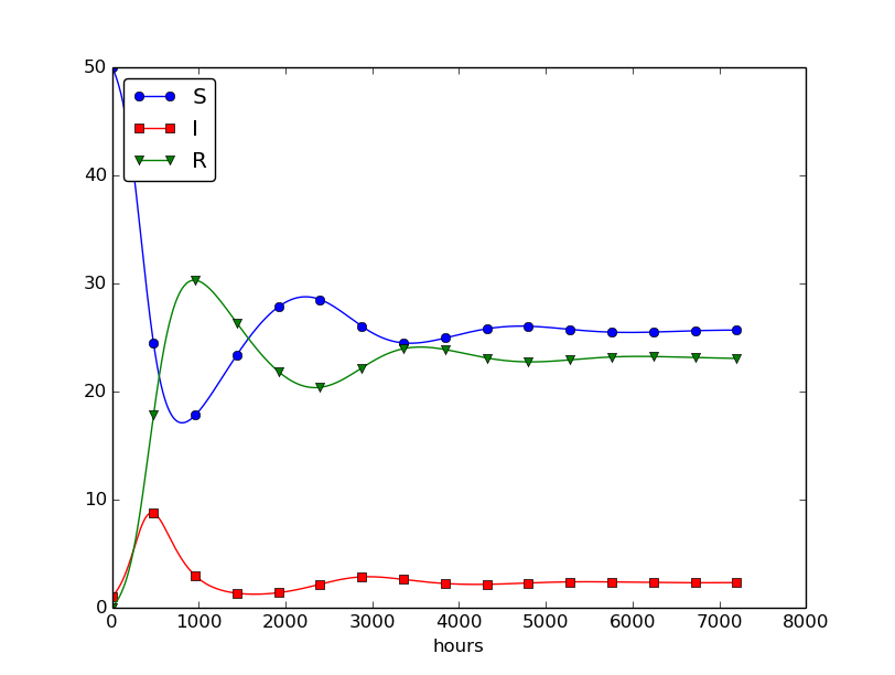
Including loss of immunity

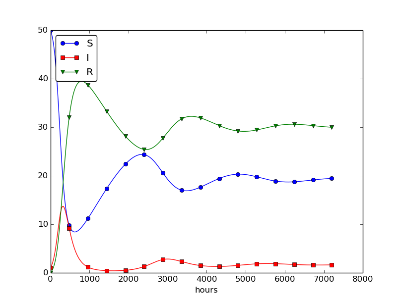
Increasing \( beta \) and reducing \( nu \) compared to Figure :ref:`sec:de:flu:fig3`

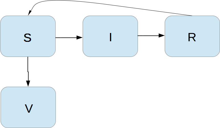
Incorporating vaccination

We can extend the model to also include vaccination. To this end, it can be useful to track those who are vaccinated and those who are not. So, we introduce a fourth category, V, for those who have taken a successful vaccination. Furthermore, we assume that in a time interval \(\Delta t\), a fraction \(p\Delta t\) of the S category is subject to a successful vaccination. This means that in the time \(\Delta t\), \(p\Delta t S\) people leave from the S to the V category. Since the vaccinated ones cannot get the disease, there is no impact on the I or R categories. We can visualize the categories, and the movement between them, as

The new, extended differential equations with the \(V\) quantity become

\[\tag{64} S' = -\beta SI + \nu R -pS,\]

\[\tag{65} V' = pS,\]

\[\tag{66} I' = \beta SI - \gamma I,\]

\[\tag{67} R' = \gamma I - \nu R\thinspace .\]

We shall refer to this model as the SIRV model.

The new equation for \(V'\) poses no difficulties when it comes to the numerical method. In a Forward Euler scheme we simply add an update

\[V^{n+1} = V^n + p \Delta t S^n\thinspace .\]

The program needs to store \(V(t)\) in an additional array V, and the plotting command must be extended with more arguments to plot V versus t as well. The complete code is found in the file SIRV1.m.

Using \(p=0.0005\) and \(p=0.0001\) as values for the vaccine efficiency parameter, the effect of vaccination is seen in Figure The effect of vaccination: \( p=0005 \) (left) and \( p=0.0001 \) (right) (other parameters are as in Figure Including loss of immunity).

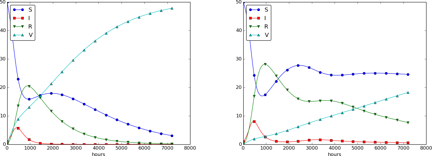
The effect of vaccination: \( p=0005 \) (left) and \( p=0.0001 \) (right)

Discontinuous coefficients: a vaccination campaign

What about modeling a vaccination campaign? Imagine that six days after the outbreak of the disease, the local health station launches a vaccination campaign. They reach out to many people, say 10 times as efficiently as in the previous (constant vaccination) case. If the campaign lasts for 10 days we can write

\[\begin{split}p(t) = \left\lbrace\begin{array}{ll} 0.005,& 6\cdot 24\leq t\leq 15\cdot 24,\\ 0,& \hbox{otherwise} \end{array}\right.\end{split}\]

Note that we must multiply the \(t\) value by 24 because \(t\) is measured in hours, not days. In the differential equation system, \(pS(t)\) must be replaced by \(p(t)S(t)\), and in this case we get a differential equation system with a term that is discontinuous. This is usually quite a challenge in mathematics, but as long as we solve the equations numerically in a program, a discontinuous coefficient is easy to treat.

There are two ways to implement the discontinuous coefficient \(p(t)\): through a function and through an array. The function approach is perhaps the easiest:

function value = p(t)
    if (6*24 <= t <= 15*24)
        value = 0.005;
    else
        value = 0;
    end
end

In the code for updating the arrays S and V we get a term p(t(n))*S(n).

We can also let \(p(t)\) be an array filled with correct values prior to the simulation. Then we need to allocate an array p of length N_t+1 and find the indices corresponding to the time period between 6 and 15 days. These indices are found from the time point divided by \(\Delta t\). That is,

p = zeros(N_t+1,1);
start_index = 6*24/dt + 1;
stop_index = 15*24/dt + 1;
p(start_index:stop_index) = 0.005;

The \(p(t)S(t)\) term in the updating formulas for \(S\) and \(V\) simply becomes p(n)*S(n). The file SIRV2.m contains a program based on filling an array p.

The effect of a vaccination campaign is illustrated in Figure The effect of a vaccination campaign. All the data are as in Figure The effect of vaccination: \( p=0005 \) (left) and \( p=0.0001 \) (right) (left), except that \(p\) is ten times stronger for a period of 10 days and \(p=0\) elsewhere.

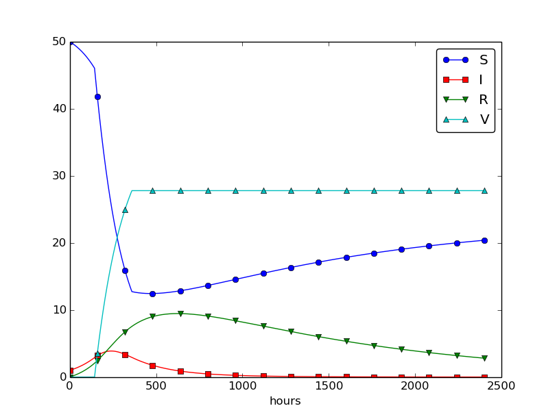
The effect of a vaccination campaign

Oscillating one-dimensional systems

Numerous engineering constructions and devices contain materials that act like springs. Such springs give rise to oscillations, and controlling oscillations is a key engineering task. We shall now learn to simulate oscillating systems.

As always, we start with the simplest meaningful mathematical model, which for oscillations is a second-order differential equation:

\[\tag{68} u''(t) + \omega^2 u(t) = 0,\]

where \(\omega\) is a given physical parameter. Equation (68) models a one-dimensional system oscillating without damping (i.e., with negligible damping). One-dimensional here means that some motion takes place along one dimension only in some coordinate system. Along with (68) we need the two initial conditions \(u(0)\) and \(u'(0)\).

Derivation of a simple model

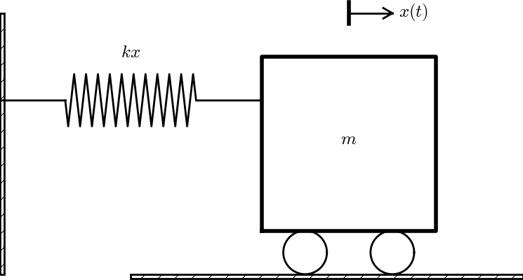
Sketch of a one-dimensional, oscillating dynamic system (without friction)

Many engineering systems undergo oscillations, and differential equations constitute the key tool to understand, predict, and control the oscillations. We start with the simplest possible model that captures the essential dynamics of an oscillating system. Some body with mass \(m\) is attached to a spring and moves along a line without friction, see Figure Sketch of a one-dimensional, oscillating dynamic system (without friction) for a sketch (rolling wheels indicate “no friction”). When the spring is stretched (or compressed), the spring force pulls (or pushes) the body back and work “against” the motion. More precisely, let \(x(t)\) be the position of the body on the \(x\) axis, along which the body moves. The spring is not stretched when \(x=0\), so the force is zero, and \(x=0\) is hence the equilibrium position of the body. The spring force is \(-kx\), where \(k\) is a constant to be measured. We assume that there are no other forces (e.g., no friction). Newton’s 2nd law of motion \(F=ma\) then has \(F=-kx\) and \(a=\ddot x\),

\[\tag{69} -kx = m\ddot x,\]

which can be rewritten as

\[\tag{70} \ddot x + \omega^2x = 0,\]

by introducing \(\omega = \sqrt{k/m}\) (which is very common).

Equation (70) is a second-order differential equation, and therefore we need two initial conditions, one on the position \(x(0)\) and one on the velocity \(x'(0)\). Here we choose the body to be at rest, but moved away from its equilibrium position:

\[x(0)=X_0,\quad x'(0)=0\thinspace .\]

The exact solution of (70) with these initial conditions is \(x(t)=X_0\cos\omega t\). This can easily be verified by substituting into (70) and checking the initial conditions. The solution tells that such a spring-mass system oscillates back and forth as described by a cosine curve.

The differential equation (70) appears in numerous other contexts. A classical example is a simple pendulum that oscillates back and forth. Physics books derive, from Newton’s second law of motion, that

\[mL\theta'' + mg\sin \theta = 0,\]

where \(m\) is the mass of the body at the end of a pendulum with length \(L\), \(g\) is the acceleration of gravity, and \(\theta\) is the angle the pendulum makes with the vertical. Considering small angles \(\theta\), \(\sin \theta\approx \theta\), and we get (70) with \(x=\theta\), \(\omega = \sqrt{g/L}\), \(x(0)=\Theta\), and \(x'(0)=0\), if \(\Theta\) is the initial angle and the pendulum is at rest at \(t=0\).

Numerical solution

We have not looked at numerical methods for handling second-order derivatives, and such methods are an option, but we know how to solve first-order differential equations and even systems of first-order equations. With a little, yet very common, trick we can rewrite (70) as a first-order system of two differential equations. We introduce \(u=x\) and \(v=x'=u'\) as two new unknown functions. The two corresponding equations arise from the definition \(v=u'\) and the original equation (70):

\[\tag{71} u' = v,\]

\[\tag{72} v' = -\omega^2 u\thinspace .\]

(Notice that we can use \(u''=v'\) to remove the second-order derivative from Newton’s 2nd law.)

We can now apply the Forward Euler method to (71)-(72), exactly as we did in the section A Forward Euler method for the differential equation system:

\[\tag{73} \frac{u^{n+1}-u^n}{\Delta t} = v^n,\]

\[\tag{74} \frac{v^{n+1}-v^n}{\Delta t} = -\omega^2 u^n,\]

resulting in the computational scheme

\[\tag{75} u^{n+1} = u^n + \Delta t\,v^n,\]

\[\tag{76} v^{n+1} = v^n -\Delta t\,\omega^2 u^n\thinspace .\]

Programming the numerical method; the special case

A simple program for (75)-(76) follows the same ideas as in the section Programming the numerical method; the special case:

omega = 2;
P = 2*pi/omega;
dt = P/20;
T = 3*P;
N_t = floor(T/dt);
t = linspace(0, N_t*dt, N_t+1);

u = zeros(N_t+1, 1);
v = zeros(N_t+1, 1);

% Initial condition
X_0 = 2;
u(1) = X_0;
v(1) = 0;

% Step equations forward in time
for n = 1:N_t
    u(n+1) = u(n) + dt*v(n);
    v(n+1) = v(n) - dt*omega^2*u(n);
end

plot(t, u, 'b-', t, X_0*cos(omega*t), 'r--');
legend('numerical', 'exact', 'Location','northwest');
xlabel('t');
print('tmp', '-dpdf');  print('tmp', '-dpng');

(See file osc_FE_special_case.m.)

Since we already know the exact solution as \(u(t)=X_0\cos\omega t\), we have reasoned as follows to find an appropriate simulation interval \([0,T]\) and also how many points we should choose. The solution has a period \(P=2\pi/\omega\). (The period \(P\) is the time difference between two peaks of the \(u(t)\sim\cos\omega t\) curve.) Simulating for three periods of the cosine function, \(T=3P\), and choosing \(\Delta t\) such that there are 20 intervals per period gives \(\Delta t=P/20\) and a total of \(N_t=T/\Delta t\) intervals. The rest of the program is a straightforward coding of the Forward Euler scheme.

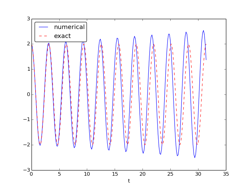
Figure Simulation of an oscillating system shows a comparison between the numerical solution and the exact solution of the differential equation. To our surprise, the numerical solution looks wrong. Is this discrepancy due to a programming error or a problem with the Forward Euler method?

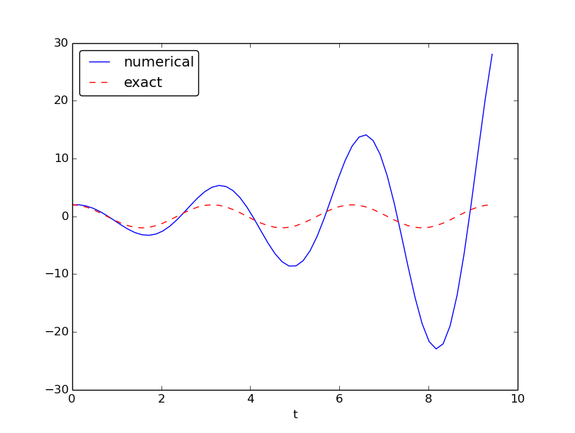
Simulation of an oscillating system

First of all, even before trying to run the program, you should sit down and compute two steps in the time loop with a calculator so you have some intermediate results to compare with. Using \(X_0=2\), \(dt=0.157079632679\), and \(\omega=2\), we get \(u^1=2\), \(v^1=-1.25663706\), \(u^2=1.80260791\), and \(v^2=-2.51327412\). Such calculations show that the program is seemingly correct. (Later, we can use such values to construct a unit test and a corresponding test function.)

The next step is to reduce the discretization parameter \(\Delta t\) and see if the results become more accurate. Figure Simulation of an oscillating system with different time steps. Upper left: 40 steps per oscillation period. Upper right: 160 steps per period. Lower left: 2000 steps per period. Lower right: 2000 steps per period, but longer simulation shows the numerical and exact solution for the cases \(\Delta t = P/40, P/160, P/2000\). The results clearly become better, and the finest resolution gives graphs that cannot be visually distinguished. Nevertheless, the finest resolution involves 6000 computational intervals in total, which is considered quite much. This is no problem on a modern laptop, however, as the computations take just a fraction of a second.

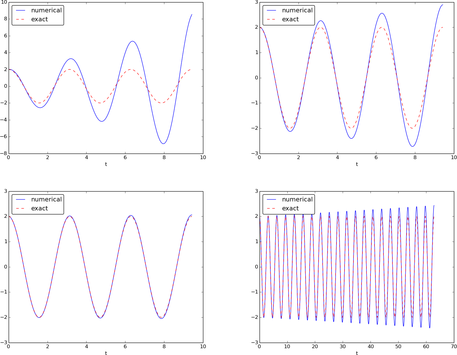
Simulation of an oscillating system with different time steps. Upper left: 40 steps per oscillation period. Upper right: 160 steps per period. Lower left: 2000 steps per period. Lower right: 2000 steps per period, but longer simulation

Although 2000 intervals per oscillation period seem sufficient for an accurate numerical solution, the lower right graph in Figure Simulation of an oscillating system with different time steps. Upper left: 40 steps per oscillation period. Upper right: 160 steps per period. Lower left: 2000 steps per period. Lower right: 2000 steps per period, but longer simulation shows that if we increase the simulation time, here to 20 periods, there is a little growth of the amplitude, which becomes significant over time. The conclusion is that the Forward Euler method has a fundamental problem with its growing amplitudes, and that a very small \(\Delta t\) is required to achieve satisfactory results. The longer the simulation is, the smaller \(\Delta t\) has to be. It is certainly time to look for more effective numerical methods!

A magic fix of the numerical method

In the Forward Euler scheme,

\[\begin{split}u^{n+1} &= u^n + \Delta t\,v^n,\\ v^{n+1} &= v^n -\Delta t\,\omega^2 u^n,\end{split}\]

we can replace \(u^n\) in the last equation by the recently computed value \(u^{n+1}\) from the first equation:

\[\tag{77} u^{n+1} = u^n + \Delta t\,v^n,\]

\[\tag{78} v^{n+1} = v^n -\Delta t\,\omega^2 u^{n+1}\thinspace .\]

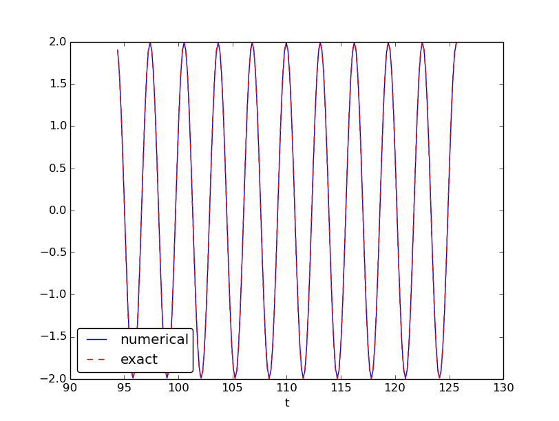
Before justifying this fix more mathematically, let us try it on the previous example. The results appear in Figure Adjusted method: first three periods (left) and period 36-40 (right). We see that the amplitude does not grow, but the phase is not entirely correct. After 40 periods (Figure Adjusted method: first three periods (left) and period 36-40 (right) right) we see a significant difference between the numerical and the exact solution. Decreasing \(\Delta t\) decreases the error. For example, with 2000 intervals per period, we only see a small phase error even after 50,000 periods (!). We can safely conclude that the fix results in an excellent numerical method!

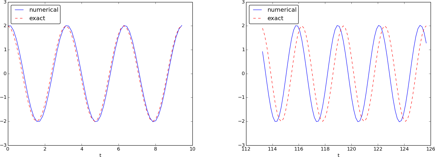
Adjusted method: first three periods (left) and period 36-40 (right)

Let us interpret the adjusted scheme mathematically. First we order (77)-(78) such that the difference approximations to derivatives become transparent:

\[\tag{79} \frac{u^{n+1} - u^n}{\Delta t} = v^n,\]

\[\tag{80} \frac{v^{n+1} - v^n}{\Delta t} = -\omega^2 u^{n+1}\thinspace .\]

We interpret (79) as the differential equation sampled at mesh point \(t_n\), because we have \(v^n\) on the right-hand side. The left-hand side is then a forward difference or Forward Euler approximation to the derivative \(u'\), see Figure Illustration of a forward difference approximation to the derivative. On the other hand, we interpret (80) as the differential equation sampled at mesh point \(t_{n+1}\), since we have \(u^{n+1}\) on the right-hand side. In this case, the difference approximation on the left-hand side is a backward difference,

\[v'(t_{n+1}) \approx \frac{v^{n+1} - v^n}{\Delta t}\quad\hbox{ or }\quad v'(t_{n}) \approx \frac{v^{n} - v^{n-1}}{\Delta t}\thinspace .\]

Figure Illustration of a backward difference approximation to the derivative illustrates the backward difference. The error in the backward difference is proportional to \(\Delta t\), the same as for the forward difference (but the proportionality constant in the error term has different sign). The resulting discretization method for (80) is often referred to as a Backward Euler scheme.

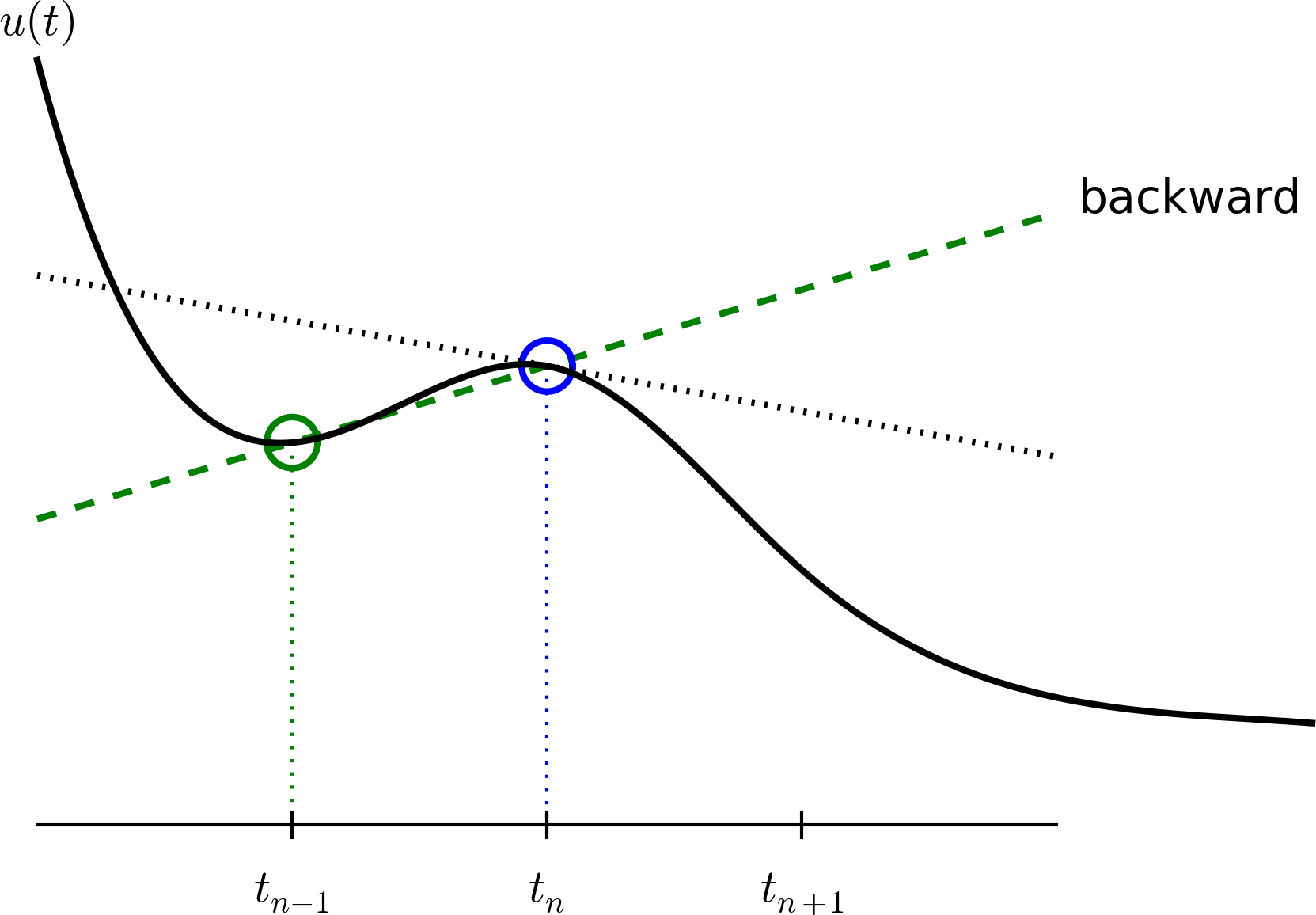
Illustration of a backward difference approximation to the derivative

To summarize, using a forward difference for the first equation and a backward difference for the second equation results in a much better method than just using forward differences in both equations.

The standard way of expressing this scheme in physics is to change the order of the equations,

\[\tag{81} v' = -\omega^2 u,\]

\[\tag{82} u' = v,\]

and apply a forward difference to (81) and a backward difference to (82):

\[\tag{83} v^{n+1} = v^n -\Delta t\,\omega^2 u^{n},\]

\[\tag{84} u^{n+1} = u^n + \Delta t\,v^{n+1}\thinspace .\]

That is, first the velocity \(v\) is updated and then the position \(u\), using the most recently computed velocity. There is no difference between (83)-(84) and (77)-(78) with respect to accuracy, so the order of the original differential equations does not matter. The scheme (83)-(84) goes under the names Semi-implicit Euler or Euler-Cromer. The implementation of (83)-(84) is found in the file osc_EC.m. The core of the code goes like

u = zeros(N_t+1,1);
v = zeros(N_t+1,1);

% Initial condition
u(1) = 2;
v(1) = 0;

% Step equations forward in time
for n = 1:N_t
    v(n+1) = v(n) - dt*omega^2*u(n);
    u(n+1) = u(n) + dt*v(n+1);
end

The 2nd-order Runge-Kutta method (or Heun’s method)

A very popular method for solving scalar and vector ODEs of first order is the 2nd-order Runge-Kutta method (RK2), also known as Heun’s method. The idea, first thinking of a scalar ODE, is to form a centered difference approximation to the derivative between two time points:

\[u'(t_n+\frac{1}{2}\Delta t)\approx \frac{u^{n+1}-u^n}{\Delta t}\thinspace .\]

The centered difference formula is visualized in Figure Illustration of a centered difference approximation to the derivative. The error in the centered difference is proportional to \(\Delta t^2\), one order higher than the forward and backward differences, which means that if we halve \(\Delta t\), the error is more effectively reduced in the centered difference since it is reduced by a factor of four rather than two.

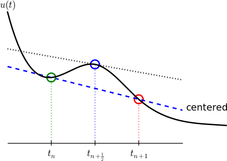
Illustration of a centered difference approximation to the derivative

The problem with such a centered scheme for the general ODE \(u'=f(u,t)\) is that we get

\[\frac{u^{n+1}-u^n}{\Delta t} = f(u^{n+\frac{1}{2}},t_{n+\frac{1}{2}}),\]

which leads to difficulties since we do not know what \(u^{n+\frac{1}{2}}\) is. However, we can approximate the value of \(f\) between two time levels by the arithmetic average of the values at \(t_n\) and \(t_{n+1}\):

\[f(u^{n+\frac{1}{2}},t_{n+\frac{1}{2}}) \approx \frac{1}{2}(f(u^n, t_n) + f(u^{n+1}, t_{n+1}))\thinspace .\]

This results in

\[\frac{u^{n+1}-u^n}{\Delta t} = \frac{1}{2}(f(u^n, t_n) + f(u^{n+1}, t_{n+1})),\]

which in general is a nonlinear algebraic equation for \(u^{n+1}\) if \(f(u,t)\) is not a linear function of \(u\). To deal with the unknown term \(f(u^{n+1}, t_{n+1})\), without solving nonlinear equations, we can approximate or predict \(u^{n+1}\) using a Forward Euler step:

\[u^{n+1} = u^n + \Delta tf(u^n,t_n)\thinspace .\]

This reasoning gives rise to the method

\[\tag{85} u^* = u^n + \Delta tf(u^n,t_n),\]

\[\tag{86} u^{n+1} = u^n + \frac{\Delta t}{2}( f(u^n,t_n) + f(u^{*},t_{n+1})\thinspace .\]

The scheme applies to both scalar and vector ODEs.

For an oscillating system with \(f=(v,-\omega^2u)\) the file osc_Heun.m implements this method. The demo script demo_osc_Heun.m runs the simulation for 10 periods with 20 time steps per period. The corresponding numerical and exact solutions are shown in Figure Simulation of 10 periods of oscillations by Heun’s method. We see that the amplitude grows, but not as much as for the Forward Euler method. However, the Euler-Cromer method is much better!

Simulation of 10 periods of oscillations by Heun’s method

We should add that in problems where the Forward Euler method gives satisfactory approximations, such as growth/decay problems or the SIR model, the 2nd-order Runge-Kutta method or Heun’s method, usually works considerably better and produces greater accuracy for the same computational cost. It is therefore a very valuable method to be aware of, although it cannot compete with the Euler-Cromer scheme for oscillation problems. The derivation of the RK2/Heun scheme is also good general training in “numerical thinking”.

Software for solving ODEs

Matlab and Octave users have a handful of functions for solving ODEs, e.g. the popular methods ode45 and ode23s. To illustrate, we may use ode45 to solve the simple problem \(u'=u\), \(u(0)=2\), for 100 time steps until \(t=4\):

u0 = 2;   % initial condition
time_points = linspace(0, 4, 101);
[t, u] = ode45(@exp_dudt, time_points, u0);

plot(t, u);
xlabel('t'); ylabel('u');

Here, ode45 is called with three parameters. The first one, @exp_dudt, is a handle to a function that specifies the right hand side of the ODE, i.e., f(u, t). In the present example, it reads

function dudt = exp_dudt(t, u)
    dudt = u

The second parameter, time_points, is an array that gives the time points on the interval where we want the solution to be reported. Alternatively, this second parameter could have been given as [0 4], which just specifies the interval, giving no directions to Matlab as to where (on the interval) the solution should be found. The third parameter, u0, just states the initial condition.

Other ODE solvers in Matlab work in a similar fashion. Several ODEs may also be solved with one function call and parameters may be included.

There is a jungle of methods for solving ODEs, and it would be nice to have easy access to implementations of a wide range of methods, especially the sophisticated and complicated adaptive methods (like ode45 and ode23s above) that adjusts \(\Delta t\) automatically to obtain a prescribed accuracy. The Python package Odespy gives easy access to a lot of numerical methods for ODEs.

The simplest possible example on using Odespy is to solve the same problem that we just looked at, i.e., \(u'=u\), \(u(0)=2\), for 100 time steps until \(t=4\):

import odespy

def f(u, t):
    return u

method = odespy.Heun   # or, e.g., odespy.ForwardEuler
solver = method(f)
solver.set_initial_condition(2)
time_points = np.linspace(0, 4, 101)
u, t = solver.solve(time_points)

In other words, you define your right-hand side function f(u, t), initialize an Odespy solver object, set the initial condition, compute a collection of time points where you want the solution, and ask for the solution. The returned arrays u and t can be plotted directly: plot(t, u).

Warning

Note that Odespy must be operated from Python, so you need to learn some basic Python to make use of this software. The type of Python programming you need to learn has a syntax very close to that of Matlab.

A nice feature of Odespy is that problem parameters can be arguments to the user’s f(u, t) function. For example, if our ODE problem is \(u'=-au+b\), with two problem parameters \(a\) and \(b\), we may write our f function as

def f(u, t, a, b):
    return -a*u + b

The extra, problem-dependent arguments a and b can be transferred to this function if we collect their values in a list or tuple when creating the Odespy solver and use the f_args argument:

a = 2
b = 1
solver = method(f, f_args=[a, b])

This is a good feature because problem parameters must otherwise be global variables - now they can be arguments in our right-hand side function in a natural way. Exercise 58: Use Odespy to solve a simple ODE asks you to make a complete implementation of this problem and plot the solution.

Using Odespy to solve oscillation ODEs like \(u''+\omega^2u=0\), reformulated as a system \(u'=v\) and \(v'=-\omega^2u\), is done as follows. We specify a given number of time steps per period and compute the associated time steps and end time of the simulation (T), given a number of periods to simulate:

import odespy

# Define the ODE system
# u' = v
# v' = -omega**2*u

def f(sol, t, omega=2):
    u, v = sol
    return [v, -omega**2*u]

# Set and compute problem dependent parameters
omega = 2
X_0 = 1
number_of_periods = 40
time_intervals_per_period = 20
from numpy import pi, linspace, cos
P = 2*pi/omega                      # length of one period
dt = P/time_intervals_per_period    # time step
T = number_of_periods*P             # final simulation time

# Create Odespy solver object
odespy_method = odespy.RK2
solver = odespy_method(f, f_args=[omega])

# The initial condition for the system is collected in a list
solver.set_initial_condition([X_0, 0])

# Compute the desired time points where we want the solution
N_t = int(round(T/dt))              # no of time intervals
time_points = linspace(0, T, N_t+1)

# Solve the ODE problem
sol, t = solver.solve(time_points)

# Note: sol contains both displacement and velocity
# Extract original variables
u = sol[:,0]
v = sol[:,1]

The last two statements are important since our two functions \(u\) and \(v\) in the ODE system are packed together in one array inside the Odespy solver. The solution of the ODE system is returned as a two-dimensional array where the first column (sol[:,0]) stores \(u\) and the second (sol[:,1]) stores \(v\). Plotting \(u\) and \(v\) is a matter of running plot(t, u, t, v).

Remark

In the right-hand side function we write f(sol, t, omega) instead of f(u, t, omega) to indicate that the solution sent to f is a solution at time t where the values of \(u\) and \(v\) are packed together: sol = [u, v]. We might well use u as argument:

def f(u, t, omega=2):
    u, v = u
    return [v, -omega**2*u]

This just means that we redefine the name u inside the function to mean the solution at time t for the first component of the ODE system.

To switch to another numerical method, just substitute RK2 by the proper name of the desired method. Typing pydoc odespy in the terminal window brings up a list of all the implemented methods. This very simple way of choosing a method suggests an obvious extension of the code above: we can define a list of methods, run all methods, and compare their \(u\) curves in a plot. As Odespy also contains the Euler-Cromer scheme, we rewrite the system with \(v'=-\omega^2u\) as the first ODE and \(u'=v\) as the second ODE, because this is the standard choice when using the Euler-Cromer method (also in Odespy):

def f(u, t, omega=2):
    v, u = u
    return [-omega**2*u, v]

This change of equations also affects the initial condition: the first component is zero and second is X_0 so we need to pass the list [0, X_0] to solver.set_initial_condition.

The code ode_odespy.py contains the details:

def compare(odespy_methods,
            omega,
            X_0,
            number_of_periods,
            time_intervals_per_period=20):

    from numpy import pi, linspace, cos
    P = 2*pi/omega                      # length of one period
    dt = P/time_intervals_per_period
    T = number_of_periods*P

    # If odespy_methods is not a list, but just the name of
    # a single Odespy solver, we wrap that name in a list
    # so we always have odespy_methods as a list
    if type(odespy_methods) != type([]):
        odespy_methods = [odespy_methods]

    # Make a list of solver objects
    solvers = [method(f, f_args=[omega]) for method in
               odespy_methods]
    for solver in solvers:
        solver.set_initial_condition([0, X_0])

    # Compute the time points where we want the solution
    dt = float(dt)  # avoid integer division
    N_t = int(round(T/dt))
    time_points = linspace(0, N_t*dt, N_t+1)

    legends = []
    for solver in solvers:
        sol, t = solver.solve(time_points)
        v = sol[:,0]
        u = sol[:,1]

        # Plot only the last p periods
        p = 6
        m = p*time_intervals_per_period  # no time steps to plot
        plot(t[-m:], u[-m:])
        hold('on')
        legends.append(solver.name())
        xlabel('t')
    # Plot exact solution too
    plot(t[-m:], X_0*cos(omega*t)[-m:], 'k--')
    legends.append('exact')
    legend(legends, loc='lower left')
    axis([t[-m], t[-1], -2*X_0, 2*X_0])
    title('Simulation of %d periods with %d intervals per period'
          % (number_of_periods, time_intervals_per_period))
    savefig('tmp.pdf'); savefig('tmp.png')
    show()

A new feature in this code is the ability to plot only the last p periods, which allows us to perform long time simulations and watch the end results without a cluttered plot with too many periods. The syntax t[-m:] plots the last m elements in t (a negative index in Python arrays/lists counts from the end).

We may compare Heun’s method (or equivalently the RK2 method) with the Euler-Cromer scheme:

compare(odespy_methods=[odespy.Heun, odespy.EulerCromer],
        omega=2, X_0=2, number_of_periods=20,
        time_intervals_per_period=20)

Figure Illustration of the impact of resolution (time steps per period) and length of simulation shows how Heun’s method (the blue line with small disks) has considerable error in both amplitude and phase already after 14-20 periods (upper left), but using three times as many time steps makes the curves almost equal (upper right). However, after 194-200 periods the errors have grown (lower left), but can be sufficiently reduced by halving the time step (lower right).

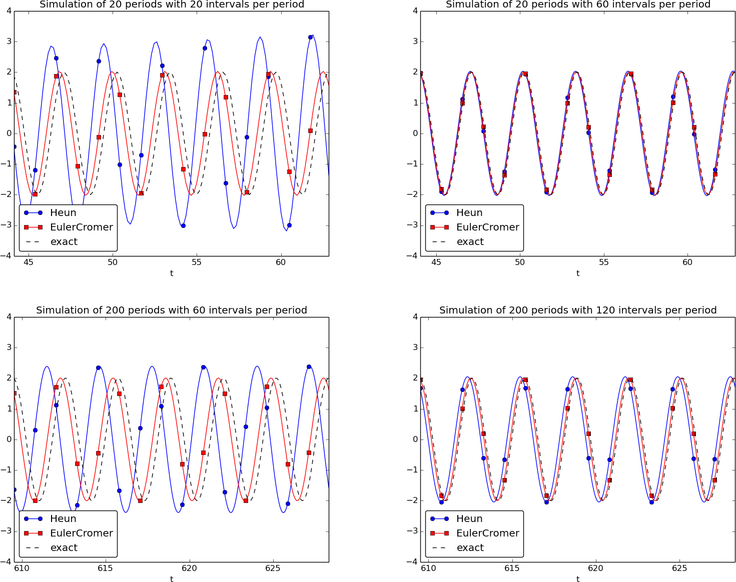
Illustration of the impact of resolution (time steps per period) and length of simulation

With all the methods in Odespy at hand, it is now easy to start exploring other methods, such as backward differences instead of the forward differences used in the Forward Euler scheme. Exercise 59: Set up a Backward Euler scheme for oscillations addresses that problem.

Odespy contains quite sophisticated adaptive methods where the user is “guaranteed” to get a solution with prescribed accuracy. There is no mathematical guarantee, but the error will for most cases not deviate significantly from the user’s tolerance that reflects the accuracy. A very popular method of this type is the Runge-Kutta-Fehlberg method, which runs a 4th-order Runge-Kutta method and uses a 5th-order Runge-Kutta method to estimate the error so that \(\Delta t\) can be adjusted to keep the error below a tolerance. This method is also widely known as ode45, because that is the name of the function implementing the method in Matlab. We can easily test the Runge-Kutta-Fehlberg method as soon as we know the corresponding Odespy name, which is RKFehlberg:

compare(odespy_methods=[odespy.EulerCromer, odespy.RKFehlberg],
        omega=2, X_0=2, number_of_periods=200,
        time_intervals_per_period=40)

Note that the time_intervals_per_period argument refers to the time points where we want the solution. These points are also the ones used for numerical computations in the odespy.EulerCromer solver, while the odespy.RKFehlberg solver will use an unknown set of time points since the time intervals are adjusted as the method runs. One can easily look at the points actually used by the method as these are available as an array solver.t_all (but plotting or examining the points requires modifications inside the compare method).

Figure Comparison of the Runge-Kutta-Fehlberg adaptive method against the Euler-Cromer scheme for a long time simulation (200 periods) shows a computational example where the Runge-Kutta-Fehlberg method is clearly superior to the Euler-Cromer scheme in long time simulations, but the comparison is not really fair because the Runge-Kutta-Fehlberg method applies about twice as many time steps in this computation and performs much more work per time step. It is quite a complicated task to compare two so different methods in a fair way so that the computational work versus accuracy is scientifically well reported.

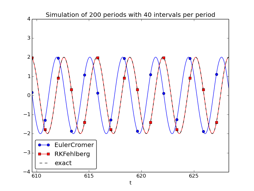
Comparison of the Runge-Kutta-Fehlberg adaptive method against the Euler-Cromer scheme for a long time simulation (200 periods)

The 4th-order Runge-Kutta method

The 4th-order Runge-Kutta method (RK4) is clearly the most widely used method to solve ODEs. Its power comes from high accuracy even with not so small time steps.

The algorithm

We first just state the four-stage algorithm:

\[\tag{87} u^{n+1} = u^n + \frac{\Delta t}{6}\left( f^n + 2\hat{f}^{n+\frac{1}{2}} + 2\tilde{f}^{n+\frac{1}{2}} + \bar{f}^{n+1}\right),\]

where

\[\tag{88} \hat{f}^{n+\frac{1}{2}} = f(u^n + \frac{1}{2}{\Delta t} f^n, t_{n+\frac{1}{2}}),\]

\[\tag{89} \tilde{f}^{n+\frac{1}{2}} = f(u^n + \frac{1}{2}\Delta t\hat{f}^{n+\frac{1}{2}}, t_{n+\frac{1}{2}}),\]

\[\tag{90} \bar{f}^{n+1} = f(u^n + \Delta t \tilde{f}^{n+\frac{1}{2}}, t_{n+1})\thinspace .\]

Application

We can run the same simulation as in Figures Simulation of an oscillating system, Adjusted method: first three periods (left) and period 36-40 (right), and Simulation of 10 periods of oscillations by Heun’s method, for 40 periods. The 10 last periods are shown in Figure The last 10 of 40 periods of oscillations by the 4th-order Runge-Kutta method. The results look as impressive as those of the Euler-Cromer method.

The last 10 of 40 periods of oscillations by the 4th-order Runge-Kutta method

Implementation

The stages in the 4th-order Runge-Kutta method can easily be implemented as a modification of the osc_Heun.py code. Alternatively, one can use the osc_odespy.py code by just providing the argument odespy_methods=[odespy.RK4] to the compare function.

Derivation

The derivation of the 4th-order Runge-Kutta method can be presented in a pedagogical way that brings many fundamental elements of numerical discretization techniques together and that illustrates many aspects of “numerical thinking” when constructing approximate solution methods.

We start with integrating the general ODE \(u'=f(u,t)\) over a time step, from \(t_n\) to \(t_{n+1}\),

\[u(t_{n+1}) - u(t_n) = \int\limits_{t_{n}}^{t_{n+1}} f(u(t),t)dt\thinspace .\]

The goal of the computation is \(u(t_{n+1})\) (\(u^{n+1}\)), while \(u(t_n)\) (\(u^n\)) is the most recently known value of \(u\). The challenge with the integral is that the integrand involves the unknown \(u\) between \(t_n\) and \(t_{n+1}\).

The integral can be approximated by the famous Simpson’s rule:

\[\int\limits_{t_{n}}^{t_{n+1}} f(u(t),t)dt \approx \frac{\Delta t}{6}\left( f^n + 4f^{n+\frac{1}{2}} + f^{n+1}\right)\thinspace .\]

The problem with this formula is that we do not know \(f^{n+\frac{1}{2}}=f(u^{n+\frac{1}{2}},t_{n+\frac{1}{2}})\) and \(f^{n+1}=(u^{n+1},t_{n+1})\) as only \(u^n\) is available and only \(f^n\) can then readily be computed.

To proceed, the idea is to use various approximations for \(f^{n+\frac{1}{2}}\) and \(f^{n+1}\) based on using well-known schemes for the ODE in the intervals \([t_n,t_{n+\frac{1}{2}}]\) and \([t_n, t_{n+1}]\). Let us split the integral into four terms:

\[\int\limits_{t_{n}}^{t_{n+1}} f(u(t),t)dt \approx \frac{\Delta t}{6}\left( f^n + 2\hat{f}^{n+\frac{1}{2}} + 2\tilde{f}^{n+\frac{1}{2}} + \bar{f}^{n+1}\right),\]

where \(\hat{f}^{n+\frac{1}{2}}\), \(\tilde{f}^{n+\frac{1}{2}}\), and \(\bar{f}^{n+1}\) are approximations to \(f^{n+\frac{1}{2}}\) and \(f^{n+1}\) that can utilize already computed quantities. For \(\hat{f}^{n+\frac{1}{2}}\) we can simply apply an approximation to \(u^{n+\frac{1}{2}}\) based on a Forward Euler step of size \(\frac{1}{2}\Delta t\):

\[\tag{91} \hat{f}^{n+\frac{1}{2}} = f(u^n + \frac{1}{2}{\Delta t} f^n, t_{n+\frac{1}{2}})\]

This formula provides a prediction of \(f^{n+\frac{1}{2}}\), so we can for \(\tilde{f}^{n+\frac{1}{2}}\) try a Backward Euler method to approximate \(u^{n+\frac{1}{2}}\):

\[\tag{92} \tilde{f}^{n+\frac{1}{2}} = f(u^n + \frac{1}{2}\Delta t\hat{f}^{n+\frac{1}{2}}, t_{n+\frac{1}{2}})\thinspace .\]

With \(\tilde{f}^{n+\frac{1}{2}}\) as an approximation to \(f^{n+\frac{1}{2}}\), we can for the final term \(\bar{f}^{n+1}\) use a midpoint method (or central difference, also called a Crank-Nicolson method) to approximate \(u^{n+1}\):

\[\tag{93} \bar{f}^{n+1} = f(u^n + \Delta t \hat{f}^{n+\frac{1}{2}}, t_{n+1})\thinspace .\]

We have now used the Forward and Backward Euler methods as well as the centered difference approximation in the context of Simpson’s rule. The hope is that the combination of these methods yields an overall time-stepping scheme from \(t_n\) to \(t_n{+1}\) that is much more accurate than the individual steps which have errors proportional to \(\Delta t\) and \(\Delta t^2\). This is indeed true: the numerical error goes in fact like \(C\Delta t^4\) for a constant \(C\), which means that the error approaches zero very quickly as we reduce the time step size, compared to the Forward Euler method (error \(\sim\Delta t\)), the Euler-Cromer method (error \(\sim\Delta t^2\)) or the 2nd-order Runge-Kutta, or Heun’s, method (error \(\sim\Delta t^2\)).

Note that the 4th-order Runge-Kutta method is fully explicit so there is never any need to solve linear or nonlinear algebraic equations, regardless of what \(f\) looks like. However, the stability is conditional and depends on \(f\). There is a large family of implicit Runge-Kutta methods that are unconditionally stable, but require solution of algebraic equations involving \(f\) at each time step. The Odespy package has support for a lot of sophisticated explicit Runge-Kutta methods, but not yet implicit Runge-Kutta methods.

More effects: damping, nonlinearity, and external forces

Our model problem \(u''+\omega^2u=0\) is the simplest possible mathematical model for oscillating systems. Nevertheless, this model makes strong demands to numerical methods, as we have seen, and is very useful as a benchmark for evaluating the performance of numerical methods.

Real-life applications involve more physical effects, which lead to a differential equation with more terms and also more complicated terms. Typically, one has a damping force \(f(u')\) and a spring force \(s(u)\). Both these forces may depend nonlinearly on their argument, \(u'\) or \(u\). In addition, environmental forces \(F(t)\) may act on the system. For example, the classical pendulum has a nonlinear “spring” or restoring force \(s(u)\sim \sin(u)\), and air resistance on the pendulum leads to a damping force \(f(u')\sim |u'|u'\). Examples on environmental forces include shaking of the ground (e.g., due to an earthquake) as well as forces from waves and wind.

With three types of forces on the system: \(F\), \(f\), and \(s\), the sum of forces is written \(F(t) - f(u') - s(u)\). Note the minus sign in front of \(f\) and \(s\), which indicates that these functions are defined such that they represent forces acting against the motion. For example, springs attached to the wheels in a car are combined with effective dampers, each providing a damping force \(f(u')=bu'\) that acts against the spring velocity \(u'\). The corresponding physical force is then \(-f\): \(-bu'\), which points downwards when the spring is being stretched (and \(u'\) points upwards), while \(-f\) acts upwards when the spring is being compressed (and \(u'\) points downwards).

Figure General oscillating system shows an example of a mass \(m\) attached to a potentially nonlinear spring and dashpot, and subject to an environmental force \(F(t)\). Nevertheless, our general model can equally well be a pendulum as in Figure A pendulum with forces with \(s(u)=mg\sin\theta\) and \(f(\dot u) =\frac{1}{2}C_D A\varrho \dot\theta |\dot\theta|\) (where \(C_D=0.4\), \(A\) is the cross sectional area of the body, and \(\varrho\) is the density of air).

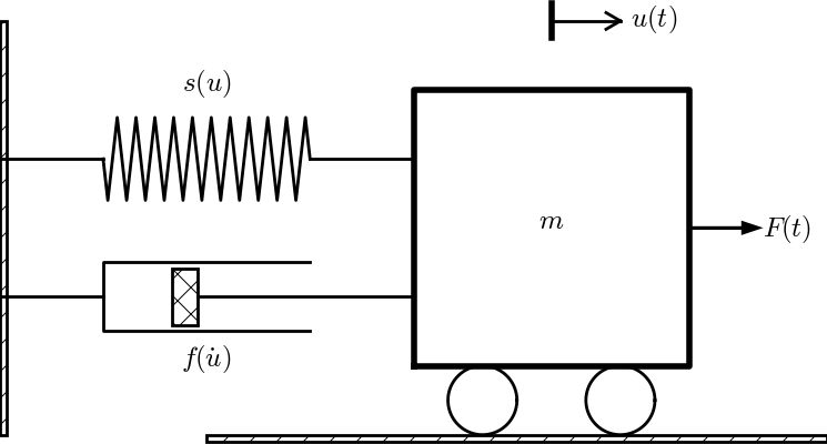
General oscillating system

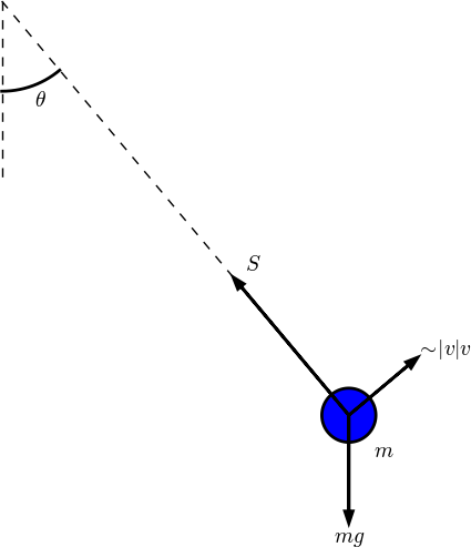
A pendulum with forces

Newton’s second law for the system can be written with the mass times acceleration on the left-hand side and the forces on the right-hand side:

\[mu'' = F(t) - f(u') - s(u)\thinspace .\]

This equation is, however, more commonly reordered to

\[\tag{94} mu'' + f(u') + s(u) = F(t)\thinspace .\]

Because the differential equation is of second order, due to the term \(u''\), we need two initial conditions:

\[\tag{95} u(0)=U_0,\quad u'(0)=V_0\thinspace .\]

Note that with the choices \(f(u')=0\), \(s(u)=ku\), and \(F(t)=0\) we recover the original ODE \(u'' +\omega^2u=0\) with \(\omega=\sqrt{k/m}\).

How can we solve (94)? As for the simple ODE \(u''+\omega^2u=0\), we start by rewriting the second-order ODE as a system of two first-order ODEs:

\[\tag{96} v' = \frac{1}{m}\left(F(t) - s(u) - f(v)\right),\]

\[\tag{97} u' = v\thinspace .\]

The initial conditions become \(u(0)=U_0\) and \(v(0)=V_0\).

Any method for a system of first-order ODEs can be used to solve for \(u(t)\) and \(v(t)\).

The Euler-Cromer scheme

An attractive choice from an implementational, accuracy, and efficiency point of view is the Euler-Cromer scheme where we take a forward difference in (96) and a backward difference in (97):

\[\tag{98} \frac{v^{n+1}-v^n}{\Delta t} = \frac{1}{m}\left(F(t_n) - s(u^n) - f(v^n)\right),\]

\[\tag{99} \frac{u^{n+1}-u^n}{\Delta t} = v^{n+1},\]

We can easily solve for the new unknowns \(v^{n+1}\) and \(u^{n+1}\):

\[\tag{100} v^{n+1} = v^n + \frac{\Delta t}{m}\left(F(t_n) - s(u^n) - f(v^n)\right),\]

\[\tag{101} u^{n+1} = u^n + \Delta t v^{n+1}\thinspace .\]

Remark on the ordering of the ODEs

The ordering of the ODEs in the ODE system is important for the extended model (96)-(97). Imagine that we write the equation for \(u'\) first and then the one for \(v'\). The Euler-Cromer method would then first use a forward difference for \(u^{n+1}\) and then a backward difference for \(v^{n+1}\). The latter would lead to a nonlinear algebraic equation for \(v^{n+1}\),

\[v^{n+1} + \frac{\Delta t}{m}f(v^{n+1}) = v^n + \frac{\Delta t}{m}\left(F(t_{n+1}) - s(u^{n+1})\right),\]

if \(f(v)\) is a nonlinear function of \(v\). This would require a numerical method for nonlinear algebraic equations to find \(v^{n+1}\), while updating \(v^{n+1}\) through a forward difference gives an equation for \(v^{n+1}\) that is linear and trivial to solve by hand.

We can implement the Euler-Cromer method like this:

function [u_values, v_values, t_values] =...
                   EulerCromer(f, s, F, m, T, U_0, V_0, dt)
    N_t = floor(round(T/dt));
    fprintf('N_t: %d', N_t);
    t = linspace(0, N_t*dt, T_t+1);

    u = zeros(N_t+1,1);
    v = zeros(N_t+1,1);

    % Initial conditions
    u(1) = U_0;
    v(1) = V_0;

    % Step equations forward in time
    for n = 1:N_t
        v(n+1) = v(n) + dt*(1/m)*(F(t(n)) - f(v(n)) - s(u(n)));
        u(n+1) = u(n) + dt*v(n+1);
    end
    u_values = u;
    v_values = v;
    t_values = t;
end

The 4-th order Runge-Kutta method

The RK4 method just evaluates the right-hand side of the ODE system,

\[(\frac{1}{m}\left(F(t) - s(u) - f(v)\right), v)\]

for known values of \(u\), \(v\), and \(t\), so the method is very simple to use regardless of how the functions \(s(u)\) and \(f(v)\) are chosen.

Illustration of linear damping

We consider an engineering system with a linear spring, \(s(u)=kx\), and a viscous damper, where the damping force is proportional to \(u'\), \(f(u')=bu'\), for some constant \(b>0\). This choice may model the vertical spring system in a car (but engineers often like to illustrate such a system by a horizontal moving mass like the one depicted in Figure General oscillating system). We may choose simple values for the constants to illustrate basic effects of damping (and later excitations). Choosing the oscillations to be the simple \(u(t)=\cos t\) function in the undamped case, we may set \(m=1\), \(k=1\), \(b=0.3\), \(U_0=1\), \(V_0=0\). The following function implements this case:

function linear_damping()
    b = 0.3;
    f = @(v) b*v;
    s = @(u) k*u;
    F = @(t) 0;

    m = 1;
    k = 1;
    U_0 = 1;
    V_0 = 0;

    T = 12*pi;
    dt = T/5000;

    [u, v, t] = EulerCromer(f, s, F, m, T, U_0, V_0, dt);

    plot_u(u, t);
end

The plot_u function is a collection of plot statements for plotting \(u(t)\), or a part of it. Figure Effect of linear damping shows the effect of the \(bu'\) term: we have oscillations with (an approximate) period \(2\pi\), as expected, but the amplitude is efficiently damped.

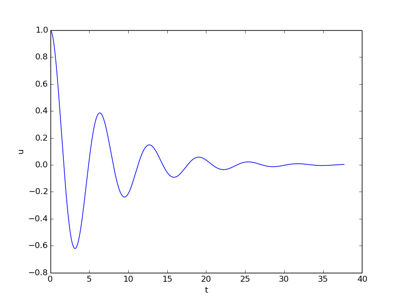
Effect of linear damping

Remark about working with a scaled problem

Instead of setting \(b=0.3\) and \(m=k=U_0=1\) as fairly “unlikely” physical values, it would be better to scale the equation \(mu'' +bu' + ku = 0\). This means that we introduce dimensionless independent and dependent variables:

\[\bar t = \frac{t}{t_c},\quad \bar u = \frac{u}{u_c},\]

where \(t_c\) and \(u_c\) are characteristic sizes of time and displacement, respectively, such that \(\bar t\) and \(\bar u\) have their typical size around unity. In the present problem, we can choose \(u_c=U_0\) and \(t_c = \sqrt{m/k}\). This gives the following scaled (or dimensionless) problem for the dimensionless quantity \(\bar u(\bar t)\):

\[\frac{d^2\bar u}{d\bar t^2} + \beta\frac{d\bar u}{d\bar t} + \bar u = 0,\quad \bar u(0)=1,\ \bar u'(0)=0,\quad \beta = \frac{b}{\sqrt{mk}} \thinspace .\]

The striking fact is that there is only one physical parameter in this problem: the dimensionless number \(\beta\). Solving this problem corresponds to solving the original problem (with dimensions) with the parameters \(m=k=U_0=1\) and \(b=\beta\). However, solving the dimensionless problem is more general: if we have a solution \(\bar u(\bar t;\beta)\), we can find the physical solution of a range of problems since

\[u(t) = U_0\bar u(t\sqrt{k/m}; \beta)\thinspace .\]

As long as \(\beta\) is fixed, we can find \(u\) for any \(U_0\), \(k\), and \(m\) from the above formula! In this way, a time consuming simulation can be done only once, but still provide many solutions. This demonstrates the power of working with scaled or dimensionless problems.

Illustration of linear damping with sinusoidal excitation

We now extend the previous example to also involve some external oscillating force on the system: \(F(t)=A\sin (wt)\). Driving a car on a road with sinusoidal bumps might give such an external excitation on the spring system in the car (\(w\) is related to the velocity of the car).

With \(A=0.5\) and \(w=3\),

w = 3;
A = 0.5;
F = @(t) A*sin(w*t);

we get the graph in Figure Effect of linear damping in combination with a sinusoidal external force. The striking difference from Figure Effect of linear damping is that the oscillations start out as a damped \(\cos t\) signal without much influence of the external force, but then the free oscillations of the undamped system (\(\cos t\)) \(u'' + u = 0\) die out and the external force \(0.5\sin(3t)\) induces oscillations with a shorter period \(2\pi/3\). You are encouraged to play around with a larger \(A\) and switch from a sine to a cosine in \(F\) and observe the effects. If you look this up in a physics book, you can find exact analytical solutions to the differential equation problem in these cases.

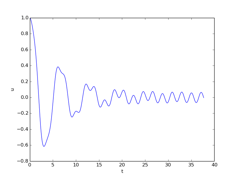
Effect of linear damping in combination with a sinusoidal external force

A particularly interesting case arises when the excitation force has the same frequency as the free oscillations of the undamped system, i.e., \(F(t)=A\sin t\). With the same amplitude \(A=0.5\), but a smaller damping \(b=0.1\), the oscillations in Figure Effect of linear damping in combination with a sinusoidal external force becomes qualitatively very different as the amplitude grows significantly larger over some periods. This phenomenon is called resonance and is exemplified in Figure Excitation force that causes resonance. Removing the damping results in an amplitude that grows linearly in time.

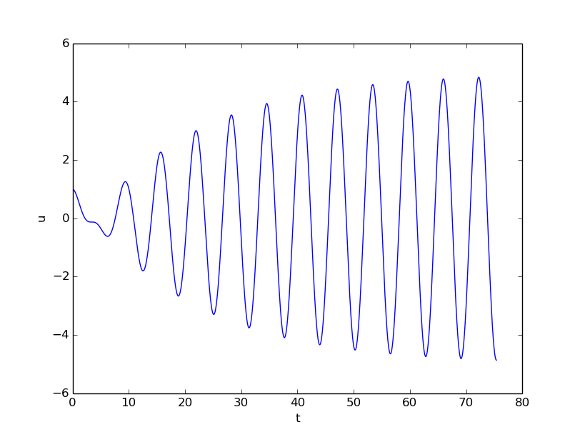
Excitation force that causes resonance

Spring-mass system with sliding friction

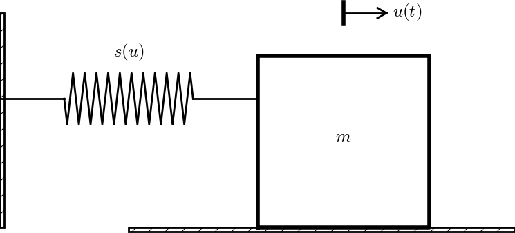
Sketch of a one-dimensional, oscillating dynamic system subject to sliding friction and a spring force

A body with mass \(m\) is attached to a spring with stiffness \(k\) while sliding on a plane surface. The body is also subject to a friction force \(f(u')\) due to the contact between the body and the plane. Figure Sketch of a one-dimensional, oscillating dynamic system subject to sliding friction and a spring force depicts the situation. The friction force \(f(u')\) can be modeled by Coulomb friction:

\[\begin{split}f(u') = \left\lbrace\begin{array}{ll} -\mu mg,& u' < 0,\\ \mu mg, & u' > 0,\\ 0, & u'=0 \end{array}\right.\end{split}\]

where \(\mu\) is the friction coefficient, and \(mg\) is the normal force on the surface where the body slides. This formula can also be written as \(f(u')=\mu mg\,\mbox{sign}(u')\), provided the signum function \(\mbox{sign}(x)\) is defined to be zero for \(x=0\) (the sign function in Matlab` has this property). To check that the signs in the definition of \(f\) are right, recall that the actual physical force is \(-f\) and this is positive (i.e., \(f<0\)) when it works against the body moving with velocity \(u'<0\).

The nonlinear spring force is taken as

\[s(u) = -k\alpha^{-1}\tanh (\alpha u),\]

which is approximately \(-ku\) for small \(u\), but stabilizes at \(\pm k/\alpha\) for large \(\pm \alpha u\). Here is a plot with \(k=1000\) and \(u\in [-0.1,0.1]\) for three \(\alpha\) values:

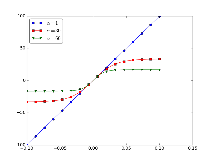
If there is no external excitation force acting on the body, we have the equation of motion

\[mu'' + \mu mg\,\mbox{sign}(u') + k\alpha^{-1}\tanh(\alpha u) = 0\thinspace .\]

Let us simulate a situation where a body of mass 1 kg slides on a surface with \(\mu =0.4\), while attached to a spring with stiffness \(k=1000\) $hbox{kg}/hbox{s}^2$. The initial displacement of the body is 10 cm, and the \(\alpha\) parameter in \(s(u)\) is set to 60 1/m. Using the EulerCromer function from the EulerCromer code, we can write a function sliding_friction for solving this problem:

function sliding_friction()
    f = @(v) mu*m*g*sign(v);
    alpha = 60.0;
    s = @(u) k/alpha*tanh(alpha*u);
    F = @(t) 0;

    g = 9.81;
    mu = 0.4;
    m = 1;
    k = 1000;

    U_0 = 0.1;
    V_0 = 0;

    T = 2;
    dt = T/5000;

    [u, v, t] = EulerCromer(f, s, F, m, T, U_0, V_0, dt);

    plot_u(u, t);
end

Running the sliding_friction function gives us the results in Figure Effect of nonlinear (left) and linear (right) spring on sliding friction with \(s(u)=k\alpha^{-1}\tanh (\alpha u)\) (left) and the linearized version \(s(u)=ku\) (right).

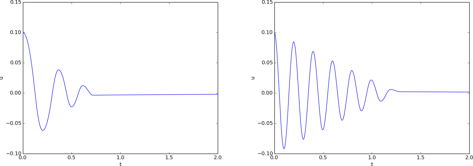
Effect of nonlinear (left) and linear (right) spring on sliding friction

A finite difference method; undamped, linear case

We shall now address numerical methods for the second-order ODE

\[u'' + \omega^2u = 0,\quad u(0)=U_0,\ u'(0)=0,\ t\in (0,T],\]

without rewriting the ODE as a system of first-order ODEs. The primary motivation for “yet another solution method” is that the discretization principles result in a very good scheme, and more importantly, the thinking around the discretization can be reused when solving partial differential equations.

The main idea of this numerical method is to approximate the second-order derivative \(u''\) by a finite difference. While there are several choices of difference approximations to first-order derivatives, there is one dominating formula for the second-order derivative:

\[\tag{102} u''(t_n) \approx \frac{u^{n+1}-2u^n + u^{n-1}}{\Delta t^2} \thinspace .\]

The error in this approximation is proportional to \(\Delta t^2\). Letting the ODE be valid at some arbitrary time point \(t_n\),

\[u''(t_n) + \omega^2 u(t_n) = 0,\]

we just insert the approximation (102) to get

\[\tag{103} \frac{u^{n+1}-2u^n + u^{n-1}}{\Delta t^2} = -\omega^2 u^n \thinspace .\]

We now assume that \(u^{n-1}\) and \(u^n\) are already computed and that \(u^{n+1}\) is the new unknown. Solving with respect to \(u^{n+1}\) gives

\[\tag{104} u^{n+1} = 2u^n - u^{n-1} - \Delta t^2\omega^2 u^n \thinspace .\]

A major problem arises when we want to start the scheme. We know that \(u^0=U_0\), but applying (104) for \(n=0\) to compute \(u^1\) leads to

\[\tag{105} u^1 = 2u^0 - u^{-1} - \Delta t^2\omega^2 u^0,\]

where we do not know \(u^{-1}\). The initial condition \(u'(0)=0\) can help us to eliminate \(u^{-1}\) - and this condition must anyway be incorporated in some way. To this end, we discretize \(u'(0)=0\) by a centered difference,

\[u'(0) \approx \frac{u^1 - u^{-1}}{2\Delta t} = 0\thinspace .\]

It follows that \(u^{-1}=u^1\), and we can use this relation to eliminate \(u^{-1}\) in (105):

\[\tag{106} u^1 = u^0 - \frac{1}{2}\Delta t^2\omega^2 u^0\thinspace .\]

With \(u^0=U_0\) and \(u^1\) computed from (106), we can compute \(u^2\), \(u^3\), and so forth from (104). Exercise 61: Discretize an initial condition asks you to explore how the steps above are modified in case we have a nonzero initial condition \(u'(0)=V_0\).

Remark on a simpler method for computing \(u^1\)

We could approximate the initial condition \(u'(0)\) by a forward difference:

\[u'(0) \approx \frac{u^1-u^0}{\Delta t} = 0,\]

leading to \(u^1=u^0\). Then we can use (104) for the coming time steps. However, this forward difference has an error proportional to \(\Delta t\), while the centered difference we used has an error proportional to \(\Delta t^2\), which is compatible with the accuracy (error goes like \(\Delta t^2\)) used in the discretization of the differential equation.

The method for the second-order ODE described above goes under the name Stormer’s method or Verlet integration. It turns out that this method is mathematically equivalent with the Euler-Cromer scheme (!). Or more precisely, the general formula (104) is equivalent with the Euler-Cromer formula, but the scheme for the first time level (106) implements the initial condition \(u'(0)\) slightly more accurately than what is naturally done in the Euler-Cromer scheme. The latter will do

\[v^1 = v^0 - \Delta t\omega^2 u^0,\quad u^1 = u^0 + \Delta t v^1 = u^0 - \Delta t^2\omega^2 u^0,\]

which differs from \(u^1\) in (106) by an amount \(\frac{1}{2}\Delta t^2\omega^2 u^0\).

Because of the equivalence of (104) with the Euler-Cromer scheme, the numerical results will have the same nice properties such as a constant amplitude. There will be a phase error as in the Euler-Cromer scheme, but this error is effectively reduced by reducing \(\Delta t\), as already demonstrated.

Another implication of the equivalence between (104) and the Euler-Cromer scheme, is that the latter must also have accuracy of order \(\Delta t^2\). One would intuitively think that using a forward and a backward difference in the Euler-Cromer scheme implies an error proportional to \(\Delta t\), but the differences are used in a symmetric way so together they form an scheme where the error is proportional to \(\Delta t^2\).

The implementation of (106) and (104) is straightforward in a function (file osc_2nd_order.m):

function [u, t] = osc_2nd_order(U_0, omega, dt, T)
    % Solve u'' + omega^2*u = 0 for t in (0,T], u(0)=U_0
    % and u'(0)=0, by a central finite difference method with
    % time step dt.
    N_t = floor(round(T/dt));
    u = zeros(N_t+1, 1);
    t = linspace(0, N_t*dt, N_t+1);

    u(1) = U_0;
    u(2) = u(1) - 0.5*dt^2*omega^2*u(1);
    for n = 2:N_t
        u(n+1) = 2*u(n) - u(n-1) - dt^2*omega^2*u(n);
    end
end

A finite difference method; linear damping

A key issue is how to generalize the scheme from the section A finite difference method; undamped, linear case to a differential equation with more terms. We start with the case of a linear damping term \(f(u')=bu'\), a possibly nonlinear spring force \(s(u)\), and an excitation force \(F(t)\):

\[\tag{107} mu'' + bu' + s(u) = F(t),\quad u(0)=U_0,\ u'(0)=0,\ t\in (0,T] \thinspace .\]

We need to find the appropriate difference approximation to \(u'\) in the \(bu'\) term. A good choice is the centered difference

\[\tag{108} u'(t_n) \approx \frac{u^{n+1}-u^{n-1}}{2\Delta t}\thinspace .\]

Sampling the equation at a time point \(t_n\),

\[mu''(t_n) + bu'(t_n) + s(u^n) = F(t_n),\]

and inserting the finite difference approximations to \(u''\) and \(u'\) results in

\[\tag{109} m\frac{u^{n+1}-2u^n + u^{n-1}}{\Delta t^2} + b\frac{u^{n+1}-u^{n-1}}{2\Delta t} + s(u^n) = F^n,\]

where \(F^n\) is a short notation for \(F(t_n)\). Equation (109) is linear in the unknown \(u^{n+1}\), so we can easily solve for this quantity:

\[\tag{110} u^{n+1} = (2mu^n + (\frac{b}{2}\Delta t - m)u^{n-1} + \Delta t^2(F^n - s(u^n)))(m + \frac{b}{2}\Delta t)^{-1}\]\[ \thinspace .\]

As in the case without damping, we need to derive a special formula for \(u^1\). The initial condition \(u'(0)=0\) implies also now that \(u^{-1}=u^1\), and with (110) for \(n=0\), we get

\[\tag{111} u^1 = u^0 + \frac{\Delta t^2}{2m}(F^0 - s(u^0)) \thinspace .\]

In the more general case with a nonlinear damping term \(f(u')\),

\[mu'' + f(u') + s(u) = F(t),\]

we get

\[m\frac{u^{n+1}-2u^n + u^{n-1}}{\Delta t^2} + f(\frac{u^{n+1}-u^{n-1}}{2\Delta t}) + s(u^n) = F^n,\]

which is a nonlinear algebraic equation for \(u^{n+1}\) that must be solved by numerical methods. A much more convenient scheme arises from using a backward difference for \(u'\),

\[u'(t_n)\approx \frac{u^n-u^{n-1}}{\Delta t},\]

because the damping term will then be known, involving only \(u^n\) and \(u^{n-1}\), and we can easily solve for \(u^{n+1}\).

The downside of the backward difference compared to the centered difference (108) is that it reduces the order of the accuracy in the overall scheme from \(\Delta t^2\) to \(\Delta t\). In fact, the Euler-Cromer scheme evaluates a nonlinear damping term as \(f(v^n)\) when computing \(v^{n+1}\), and this is equivalent to using the backward difference above. Consequently, the convenience of the Euler-Cromer scheme for nonlinear damping comes at a cost of lowering the overall accuracy of the scheme from second to first order in \(\Delta t\). Using the same trick in the finite difference scheme for the second-order differential equation, i.e., using the backward difference in \(f(u')\), makes this scheme equally convenient and accurate as the Euler-Cromer scheme in the general nonlinear case \(mu''+f(u')+s(u)=F\).

Exercises

Exercise 43: Geometric construction of the Forward Euler method

The section Understanding the Forward Euler method describes a geometric interpretation of the Forward Euler method. This exercise will demonstrate the geometric construction of the solution in detail. Consider the differential equation \(u'=u\) with \(u(0)=1\). We use time steps \(\Delta t = 1\).

a) Start at \(t=0\) and draw a straight line with slope \(u'(0)=u(0)=1\). Go one time step forward to \(t=\Delta t\) and mark the solution point on the line.

Solution. See plot and comments given below.

b) Draw a straight line through the solution point \((\Delta t, u^1)\) with slope \(u'(\Delta t)=u^1\). Go one time step forward to \(t=2\Delta t\) and mark the solution point on the line.

Solution. See plot and comments given below.

c) Draw a straight line through the solution point \((2\Delta t, u^2)\) with slope \(u'(2\Delta t)=u^2\). Go one time step forward to \(t=3\Delta t\) and mark the solution point on the line.

Solution. See plot and comments given below.

d) Set up the Forward Euler scheme for the problem \(u'=u\). Calculate \(u^1\), \(u^2\), and \(u^3\). Check that the numbers are the same as obtained in a)-c).

Solution. The code may be written as

% Forward Euler for u' = u
a = 0; b = 3;
dudt = @(u) u;
u_exact = @(t) exp(t);

u = zeros(4, 1);
u(1) = 1;
dt = 1;

for i = 1:3
    u(i+1) = u(i) + dt*dudt(u(i));
end

u
tP = [0 1 2 3];
time = linspace(a, b, 100);
u_true = u_exact(time);
plot(time, u_true, 'b-', tP, u, 'ro');
xlabel('t');
ylabel('u(t)');

Running the program will print the numbers 1, 2, 4 and 8, as well as produce the plot seen in Figure Forward Euler method (red filled circles) applied to the ode \( u’ = u \) . For easy comparison, the true solution \( u(t) = e^t \) is also shown (blue continuous line). We see the values computed in a)-c) as circles (which in a)-c) are connected by straight line segments). For comparison, the true solution is also given. The very large timestep gives a rather poor numerical solution.

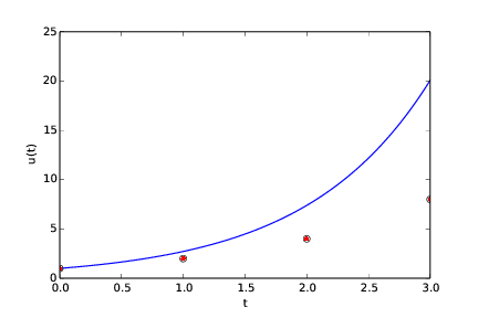
Forward Euler method (red filled circles) applied to the ode \( u’ = u \) . For easy comparison, the true solution \( u(t) = e^t \) is also shown (blue continuous line)

Filename: ForwardEuler_geometric_solution.m.

Exercise 44: Make test functions for the Forward Euler method

The purpose of this exercise is to make a file test_ode_FE.m that makes use of the ode_FE function in the file ode_FE.m and automatically verifies the implementation of ode_FE.

a) The solution computed by hand in Exercise 43: Geometric construction of the Forward Euler method can be used as a reference solution. Make a function test_ode_FE_1() that calls ode_FE to compute three time steps in the problem \(u'=u\), \(u(0)=1\), and compare the three values \(u^1\), \(u^2\), and \(u^3\) with the values obtained in Exercise 43: Geometric construction of the Forward Euler method.

Solution. See code presented below.

b) The test in a) can be made more general using the fact that if \(f\) is linear in \(u\) and does not depend on \(t\), i.e., we have \(u'=ru\), for some constant \(r\), the Forward Euler method has a closed form solution as outlined in the section Derivation of the model: \(u^n=U_0(1+r\Delta t)^n\). Use this result to construct a test function test_ode_FE_2() that runs a number of steps in ode_FE and compares the computed solution with the listed formula for \(u^n\).

Solution. The code may be written as:

function growth2_test()
    test_ode_FE_1();
    test_ode_FE_2();
end

function test_ode_FE_1()
    hand = [1 2 4 8];
    T = 3;
    dt = 1;
    U_0 = 1.0;
    function result = f(u, t)
        result = u;
    end
    [u, t] = ode_FE(@f, U_0, dt, T);
    tol = 1E-14;
    for i = 1:length(hand)
        err = abs(hand(i) - u(i));
        assert(err < tol, 'i=%d, err=%g', i, err);
    end
end

function test_ode_FE_2()
    T = 3;
    dt = 0.1;       % Tested first dt = 1.0, ok
    U_0 = 1.0;
    function result = f(u, t)
        r = 1;
        result = r*u;
    end
    function result = u_exact(U_0, dt, n)
        r = 1;
        result = U_0*(1+r*dt)^n;
    end
    [u, t] = ode_FE(@f, U_0, dt, T);
    tol = 1E-12;     % Relaxed from 1E-14 to get through
    for n = 1:length(u)
        err = abs(u_exact(U_0, dt, n-1) - u(n));
        assert(err < tol, 'n=%d, err=%g', n, err);
    end
end

Filename: test_ode_FE.m.

Exercise 45: Implement and evaluate Heun’s method

a) A 2nd-order Runge-Kutta method, also known has Heun’s method, is derived in the section The 2nd-order Runge-Kutta method (or Heun’s method). Make a function ode_Heun(f, U_0, dt, T) (as a counterpart to ode_FE(f, U_0, dt, T) in ode_FE.m) for solving a scalar ODE problem \(u'=f(u,t)\), \(u(0)=U_0\), \(t\in (0,T]\), with this method using a time step size \(\Delta t\).

Solution. The code may be written as:

function [u_found, t_used] = ode_Heun(f, U_0, dt, T)
    N_t = floor(T/dt);
    u = zeros(N_t+1, 1);
    t = linspace(0, N_t*dt, length(u));
    u(1) = U_0;
    for n = 1:N_t
        u_star = u(n) + dt*f(u(n),t(n));
        u(n+1) = u(n) + 0.5*dt*(f(u(n),t(n)) + f(u_star,t(n)));
    end
    u_found = u;
    t_used = t;
end

b) Solve the simple ODE problem \(u'=u\), \(u(0)=1\), by the ode_Heun and the ode_FE function. Make a plot that compares Heun’s method and the Forward Euler method with the exact solution \(u(t)=e^t\) for \(t\in [0,6]\). Use a time step \(\Delta t = 0.5\).

Solution. The given ODE may be solved by the function demo_ode_Heun:

function demo_ode_Heun()
    % Test case: u' = u, u(0) = 1
    function value = f(u,t)
        value = u;
    end
    U_0 = 1;
    dt = 0.5;
    T = 6;
    [u_Heun, t] = ode_Heun(@f, U_0, dt, T);
    [u_FE, t]   = ode_FE(@f, U_0, dt, T);

    plot(t, u_Heun, 'b-', t, u_FE, 'b--', t, exp(t), 'r--');
    xlabel('t');
    legend('H', 'FE', 'true', 'location', 'northwest');
end

Running the code with \(\Delta t = 0.5\) (seen in the code) gives the plot seen in Figure Heun and Forward Euler with timestep .

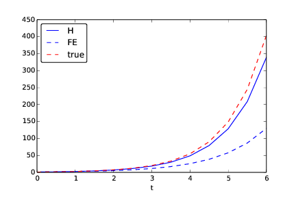
Heun and Forward Euler with timestep \(\Delta t = 0.5\)

c) For the case in b), find through experimentation the largest value of \(\Delta t\) where the exact solution and the numerical solution by Heun’s method cannot be distinguished visually. It is of interest to see how far off the curve the Forward Euler method is when Heun’s method can be regarded as “exact” (for visual purposes).

Solution. A timestep of \(\Delta t = 0.1\) was found to be the largest reasonable timestep that still made the solution from Heun’s method come on top of the exact solution (from graphical inspection only), see Figure Heun and Forward Euler with timestep \( Delta t = 0.1 \) . A larger timestep makes Heun’s method deviate from the true solution (only judged graphically).

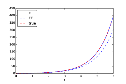
Heun and Forward Euler with timestep \( Delta t = 0.1 \) . A larger timestep makes Heun’s method deviate from the true solution (only judged graphically)

Filename: ode_Heun.m.

Exercise 46: Find an appropriate time step; logistic model

Compute the numerical solution of the logistic equation for a set of repeatedly halved time steps: \(\Delta t_k = 2^{-k}\Delta t\), \(k=0,1,\ldots\). Plot the solutions corresponding to the last two time steps \(\Delta t_{k}\) and \(\Delta t_{k-1}\) in the same plot. Continue doing this until you cannot visually distinguish the two curves in the plot. Then one has found a sufficiently small time step.

Hint. Extend the logistic.m file. Introduce a loop over \(k\), write out \(\Delta t_k\), and ask the user if the loop is to be continued.

Solution. This may be implemented as:

dt = 20; T = 100;
f = @(u,t) 0.1*(1-u/500)*u;
U_0 = 100;
[u_old, t_old] = ode_FE(f, U_0, dt, T);

k = 1;
one_more = true;
while one_more == true
    dt_k = 2^(-k)*dt;
    [u_new, t_new] = ode_FE(f, U_0, dt_k, T);
    plot(t_old, u_old, 'b-', t_new, u_new, 'r--')
    xlabel('t'); ylabel('N(t)');
    fprintf('Timestep was: %g\n', dt_k);
    answer = input('Do one more with finer dt (y/n)? ', 's')
    if strcmp(answer,'y')
        u_old = u_new;
        t_old = t_new;
    else
        one_more = false;
    end
    k = k + 1;
end

Filename: logistic_dt.m.

Exercise 47: Find an appropriate time step; SIR model

Repeat Exercise 46: Find an appropriate time step; logistic model for the SIR model.

Hint. Import the ode_FE function from the ode_system_FE module and make a modified demo_SIR function that has a loop over repeatedly halved time steps. Plot \(S\), \(I\), and \(R\) versus time for the two last time step sizes in the same plot.

Solution. This may be implemented as:

function demo_SIR()
    % Find appropriate time step for an SIR model
    function result = f(u,t)
        beta = 10/(40*8*24);
        gamma = 3/(15*24);
        S = u(1); I = u(2); R = u(3);
        result = [-beta*S*I beta*S*I - gamma*I gamma*I];
    end

    dt = 48.0;   % 48 h
    D = 30;      % Simulate for D days
    N_t = floor(D*24/dt);    % Corresponding no of hours
    T = dt*N_t;              % End time
    U_0 = [50 1 0];

    [u_old, t_old] = ode_FE(@f, U_0, dt, T);

    S_old = u_old(:,1);
    I_old = u_old(:,2);
    R_old = u_old(:,3);
    k = 1;
    one_more = true
    while one_more == true
        dt_k = 2^(-k)*dt;
        [u_new, t_new] = ode_FE(@f, U_0, dt_k, T);
        S_new = u_new(:,1);
        I_new = u_new(:,2);
        R_new = u_new(:,3);

        plot(t_old, S_old, 'b-', t_new, S_new, 'b--',...
             t_old, I_old, 'r-', t_new, I_new, 'r--',...
             t_old, R_old, 'g-', t_new, R_new, 'g--');
        xlabel('hours');
        ylabel('S (blue), I (red), R (green)');
        fprintf('Finest timestep was: %g\n', dt_k);
        answer = input('Do one more with finer dt (y/n)? ','s');
        if strcmp(answer, 'y')
            S_old = S_new;
            R_old = R_new;
            I_old = I_new;
            t_old = t_new;
            k = k + 1;
        else
            one_more = false;
        end
    end
end

Filename: SIR_dt.m.

Exercise 48: Model an adaptive vaccination campaign

In the SIRV model with time-dependent vaccination from the section Discontinuous coefficients: a vaccination campaign, we want to test the effect of an adaptive vaccination campaign where vaccination is offered as long as half of the population is not vaccinated. The campaign starts after \(\Delta\) days. That is, \(p=p_0\) if \(V<\frac{1}{2}(S^0+I^0)\) and \(t>\Delta\) days, otherwise \(p=0\).

Demonstrate the effect of this vaccination policy: choose \(\beta\), \(\gamma\), and \(\nu\) as in the section Discontinuous coefficients: a vaccination campaign, set \(p=0.001\), \(\Delta =10\) days, and simulate for 200 days.

Hint. This discontinuous \(p(t)\) function is easiest implemented as a Matlab function containing the indicated if test. You may use the file SIRV1.m as starting point, but note that it implements a time-dependent \(p(t)\) via an array.

Solution. An appropriate program is

function SIRV_p_adapt()
    % As SIRV1.py, but including time-dependent vaccination.
    % Time unit: 1 h

    beta = 10/(40*8*24);
    beta = beta/4;        % Reduce beta compared to SIR1.py
    fprintf('beta: %g\n', beta);
    gamma = 3/(15*24);
    dt = 0.1;             % 6 min
    D = 200;              % Simulate for D days
    N_t = floor(D*24/dt); % Corresponding no of hours
    nu = 1/(24*50);       % Average loss of immunity
    Delta = 10;           % Start point of campaign (in days)
    p_0 = 0.001;

    t = linspace(0, N_t*dt, N_t+1);
    S = zeros(N_t+1, 1);
    I = zeros(N_t+1, 1);
    R = zeros(N_t+1, 1);
    V = zeros(N_t+1, 1);

    function result = p(t, n)
        if (V(n) < 0.5*(S(1)+I(1)) && t > Delta*24)
            result = p_0;
        else
            result = 0;
        end
    end

    % Initial condition
    S(1) = 50;
    I(1) = 1;
    R(1) = 0;
    V(1) = 0;

    epsilon = 1e-12;
    % Step equations forward in time
    for n = 1:N_t
        S(n+1) = S(n) - dt*beta*S(n)*I(n) + dt*nu*R(n) -...
                                          dt*p(t(n),n)*S(n);
        V(n+1) = V(n) + dt*p(t(n),n)*S(n);
        I(n+1) = I(n) + dt*beta*S(n)*I(n) - dt*gamma*I(n);
        R(n+1) = R(n) + dt*gamma*I(n) - dt*nu*R(n);
        loss = (V(n+1) + S(n+1) + R(n+1) + I(n+1)) -...
                       (V(1) + S(1) + R(1) + I(1));
        if loss > epsilon
            fprintf('loss: %g\n', loss);
        end
    end

    figure();
    plot(t, S, t, I, t, R, t, V);
    legend('S', 'I', 'R', 'V', 'Location', 'northeast');
    xlabel('hours');
    % saveas() gives poor resolution in plots, use the
    % third party function export_fig to save the plot?

end

The result looks like

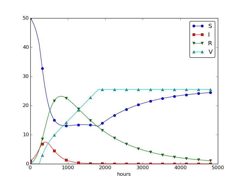
Filename: SIRV_p_adapt.m.

Exercise 49: Make a SIRV model with time-limited effect of vaccination

We consider the SIRV model from the section Incorporating vaccination, but now the effect of vaccination is time-limited. After a characteristic period of time, \(\pi\), the vaccination is no more effective and individuals are consequently moved from the V to the S category and can be infected again. Mathematically, this can be modeled as an average leakage \(-\pi^{-1}V\) from the V category to the S category (i.e., a gain \(\pi^{-1}V\) in the latter). Write up the complete model, implement it, and rerun the case from the section Incorporating vaccination with various choices of parameters to illustrate various effects. Filename: SIRV1_V2S.m.

Exercise 50: Refactor a flat program

Consider the file osc_FE.m implementing the Forward Euler method for the oscillating system model (71)-(72). The osc_FE.m is what we often refer to as a flat program, meaning that it is just one main program with no functions. To easily reuse the numerical computations in other contexts, place the part that produces the numerical solution (allocation of arrays, initializing the arrays at time zero, and the time loop) in a function osc_FE(X_0, omega, dt, T), which returns u, v, t. Place the particular computational example in osc_FE.m in a function demo(). Construct the file osc_FE_func.m such that the osc_FE function can easily be reused in other programs.

Solution. Here is the file osc_FE.m:

function [u, v, t] = osc_FE(X_0, omega, dt, T)
    N_t = floor(T/dt);
    u = zeros(N_t+1, 1);
    v = zeros(N_t+1, 1);
    t = linspace(0, N_t*dt, N_t+1);

    % Initial condition
    u(1) = X_0;
    v(1) = 0;

    % Step equations forward in time
    for n = 1:N_t
        u(n+1) = u(n) + dt*v(n);
        v(n+1) = v(n) - dt*omega^2*u(n);
    end
end

which is run from the demo file:

function demo_osc_FE()
    omega = 2;
    P = 2*pi/omega;
    dt = P/20;
    T = 3*P;
    X_0 = 2;
    [u, v, t] = osc_FE(X_0, omega, dt, T);

    plot(t, u, 'b-', t, X_0*cos(omega*t), 'r--');
    legend('numerical', 'exact', 'Location', 'nortwest');
    xlabel('t');
end

Filename: osc_FE_func.m.

Exercise 51: Simulate oscillations by a general ODE solver

Solve the system (71)-(72) using the general solver ode_FE in the file ode_system_FE.m described in the section Programming the numerical method; the general case. Program the ODE system and the call to the ode_FE function in a separate file osc_ode_FE.m.

Equip this file with a test function that reads a file with correct \(u\) values and compares these with those computed by the ode_FE function. To find correct \(u\) values, modify the program osc_FE.m to dump the u array to file, run osc_FE.m, and let the test function read the reference results from that file.

Solution. The program may be implemented as:

function test_osc_ode_FE()
    function result = f(sol, t)
        u = sol(1);  v = sol(2);
        %fprintf('dudt: %g , dvdt: %g\n', v, -omega^2*u);
        result = [v -omega^2*u];
    end

    % Set and compute problem dependent parameters
    omega = 2;
    X_0 = 1;
    number_of_periods = 6;
    time_intervals_per_period = 20;

    P = 2*pi/omega;                     % Length of one period
    dt = P/time_intervals_per_period;   % Time step
    T = number_of_periods*P;            % Final simulation time
    U_0 = [X_0 0];                      % Initial conditions

    % Produce u data on file that will be used for reference
    file_name = 'osc_FE_data';
    osc_FE_2file(file_name, X_0, omega, dt, T);

    [sol, t] = ode_FE(@f, U_0, dt, T);
    u = sol(:,1);

    % Read data from file for comparison
    infile = fopen(file_name, 'r');
    u_ref = fscanf(infile, '%f');
    fclose(infile);

    tol = 1E-5;               % Tried several stricter ones first
    for n = 1:length(u)
        err = abs(u_ref(n) - u(n));
        assert(err < tol, 'n=%d, err=%g', n, err);
    end

    % Choose to also plot, just to get a visual impression of u
    plot(t, u_ref, 'b-', t, u, 'r--');
    legend('u ref', 'u');
end

function osc_FE_2file(filename, X_0, omega, dt, T)
    N_t = floor(T/dt);
    u = zeros(N_t+1, 1);
    v = zeros(N_t+1, 1);

    % Initial condition
    u(1) = X_0;
    v(1) = 0;

    outfile = fopen(filename, 'w');
    fprintf(outfile,'%10.5f\n', u(1));

    % Step equations forward in time
    for n = 1:N_t
        u(n+1) = u(n) + dt*v(n);
        v(n+1) = v(n) - dt*omega^2*u(n);
        fprintf(outfile,'%10.5f\n', u(n+1));
    end
    fclose(outfile);
end

Filename: osc_ode_FE.m.

Exercise 52: Compute the energy in oscillations

a) Make a function osc_energy(u, v, omega) for returning the potential and kinetic energy of an oscillating system described by (71)-(72). The potential energy is taken as \(\frac{1}{2}\omega^2u^2\) while the kinetic energy is \(\frac{1}{2}v^2\). (Note that these expressions are not exactly the physical potential and kinetic energy, since these would be \(\frac{1}{2}mv^2\) and \(\frac{1}{2}ku^2\) for a model \(mx'' + kx=0\).)

Place the osc_energy in a separate file osc_energy.m such that the function can be called from other functions.

Solution. The function may be implemented as:

function [U, K] = osc_energy(u, v, omega)
    U = 0.5*omega.^2*u.^2;
    K = 0.5*v.^2;
end

b) Add a call to osc_energy in the programs osc_FE.m and osc_EC.m and plot the sum of the kinetic and potential energy. How does the total energy develop for the Forward Euler and the Euler-Cromer schemes?

Solution. The Forward Euler code reads

omega = 2;
P = 2*pi/omega;
dt = P/20;
T = 3*P;
N_t = floor(round(T/dt));
t = linspace(0, N_t*dt, N_t+1);

u = zeros(N_t+1, 1);
v = zeros(N_t+1, 1);

% Initial condition
X_0 = 2;
u(1) = X_0;
v(1) = 0;

% Step equations forward in time
for n = 1:N_t
    u(n+1) = u(n) + dt*v(n);
    v(n+1) = v(n) - dt*omega^2*u(n);
end

[U, K] = osc_energy(u, v, omega);

plot(t, U+K, 'b-');
xlabel('t');
ylabel('U+K');

The program generates the following plot showing how the energy increases with time.

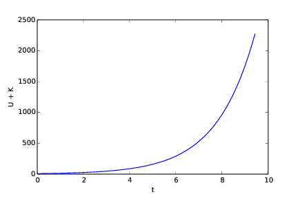
The Euler-Cromer code might be implemented as

omega = 2;
P = 2*pi/omega;
dt = P/20;
T = 40*P;
N_t = floor(round(T/dt));
t = linspace(0, N_t*dt, N_t+1);

u = zeros(N_t+1, 1);
v = zeros(N_t+1, 1);

% Initial condition
X_0 = 2;
u(1) = X_0;
v(1) = 0;

% Step equations forward in time
for n = 1:N_t
    v(n+1) = v(n) - dt*omega^2*u(n);
    u(n+1) = u(n) + dt*v(n+1);
end

[U, K] = osc_energy(u, v, omega);

plot(t, U+K, 'b-');
xlabel('t');
ylabel('U+K');

In this case, as illustrated by the plot produced, the energy does not increase.

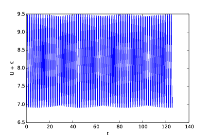
Filenames: osc_energy.m, osc_FE_energy.m, osc_EC_energy.m.

Exercise 53: Use a Backward Euler scheme for population growth

We consider the ODE problem \(N'(t)=rN(t)\), \(N(0)=N_0\). At some time, \(t_n=n\Delta t\), we can approximate the derivative \(N'(t_n)\) by a backward difference, see Figure Illustration of a backward difference approximation to the derivative:

\[N'(t_n)\approx \frac{N(t_n) - N(t_n-\Delta t)}{\Delta t} = \frac{N^n - N^{n-1}}{\Delta t},\]

which leads to

\[\frac{N^n - N^{n-1}}{\Delta t} = rN^n\thinspace,\]

called the Backward Euler scheme.

a) Find an expression for the \(N^n\) in terms of \(N^{n-1}\) and formulate an algorithm for computing \(N^n\), \(n=1,2,\ldots,N_t\).

Solution. Re-arranging the given expression leads to:

\[\tag{112} N^n = \frac{N^{n-1}}{1-r\Delta t}.\]

Noting that the right hand side may be expressed by use of \(N^0\), we may formulate the following algorithm:

For \(n = 1,2,...,N\) compute

\[\tag{113} N^n = \left(1-r\Delta t\right)^{-n} N^0.\]

b) Implement the algorithm in a) in a function growth_BE(N_0, dt, T) for solving \(N'=rN\), \(N(0)=N_0\), \(t\in (0,T]\), with time step \(\Delta t\) (dt).

Solution. Here is the code:

function N = growth_BE(r, N_0, dt, T)
    N_t = floor(round(T/dt));
    N = zeros(N_t+1, 1);
    N(1) = N_0;
    for n = 1:N_t+1
        N(n) = (1-r*dt)^(-n) * N_0;
    end
end

c) Implement the Forward Euler scheme in a function growth_FE(N_0, dt, T) as described in b).

Solution. The FE function reads:

function N = growth_FE(r, N_0, dt, T)
    N_t = floor(round(T/dt));
    N = zeros(N_t+1, 1);
    N(1) = N_0;
    for n = 1:N_t+1
        N(n) = (1+r*dt)^n * N_0;
    end
end

To use the two functions and produce the requested results, we implemented the following function:

function apply_growth_BE_and_FE()
    r = 1;
    N_0 = 1;   T = 6;
    dt = 0.5;
    N_BE = growth_BE(r, N_0, dt, T);
    N_FE = growth_FE(r, N_0, dt, T);
    time = linspace(0, T, floor(round(T/dt))+1);
    plot(time, N_BE, time, N_FE, time, exp(time));
    title('Timestep 0.5');
    legend('N (BE)', 'N (FE)', 'exp(t) (true)',...
                                 'Location', 'northwest');
    xlabel('t');
    print('tmp1', '-dpdf');

    dt = 0.05;
    N_BE = growth_BE(r, N_0, dt, T);
    N_FE = growth_FE(r, N_0, dt, T);
    time = linspace(0, T, floor(round(T/dt))+1);
    figure(), plot(time, N_BE, time, N_FE, time, exp(time));
    title('Timestep 0.05');
    legend('N (BE)', 'N (FE)', 'exp(t) (true)',...
                                 'Location', 'northwest');
    xlabel('t');
    print('tmp2', '-dpdf');
end

The two plots generated are seen below.

d) Compare visually the solution produced by the Forward and Backward Euler schemes with the exact solution when \(r=1\) and \(T=6\). Make two plots, one with \(\Delta t = 0.5\) and one with \(\Delta t=0.05\).

Solution. With a time step of 0.5, the BE approach deviates substantially more from the true solution than the FE. This is a consequence of the very large time step used.

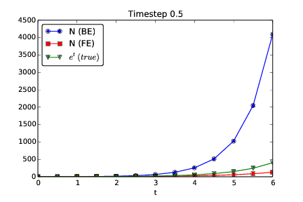
Reducing the time step to 0.05 improves the situation for BE, so that FE and BE now give approximately the same error at each time step, but with opposite signs.

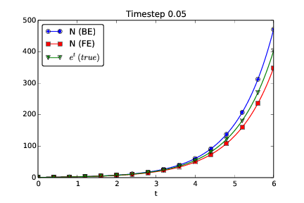
With both time steps and both methods, the error grows with time. It should be noted that the graph produced with FE is below the true solution, while the one from BE is above. This should be expected because of the following. The slope of the true graph (or solution) increases with time. The FE does, at each time step, use the derivative from the beginning of the time step. This derivative is the smallest on the time interval covered by that time step. Therefore, the corresponding graph ends up below the true one. With BE, it is the other way around, since it uses the derivative at the end of each timestep, which then is the largest derivative on the time interval covered by that time step.

Filename: growth_BE.m.

Exercise 54: Use a Crank-Nicolson scheme for population growth

It is recommended to do Exercise 53: Use a Backward Euler scheme for population growth prior to the present one. Here we look at the same population growth model \(N'(t)=rN(t)\), \(N(0)=N_0\). The time derivative \(N'(t)\) can be approximated by various types of finite differences. Exercise 53: Use a Backward Euler scheme for population growth considers a backward difference (Figure Illustration of a backward difference approximation to the derivative), while the section Numerical solution explained the forward difference (Figure Illustration of a forward difference approximation to the derivative). A centered difference is more accurate than a backward or forward difference:

\[N'(t_n+\frac{1}{2}\Delta t)\approx\frac{N(t_n+\Delta t)-N(t_n)}{\Delta t}= \frac{N^{n+1}-N^n}{\Delta t}\thinspace .\]

This type of difference, applied at the point \(t_{n+\frac{1}{2}}=t_n + \frac{1}{2}\Delta t\), is illustrated geometrically in Figure Illustration of a centered difference approximation to the derivative.

a) Insert the finite difference approximation in the ODE \(N'=rN\) and solve for the unknown \(N^{n+1}\), assuming \(N^n\) is already computed and hence known. The resulting computational scheme is often referred to as a Crank-Nicolson scheme.

Solution. With a central difference approximation used for the derivative, we also need to reformulate the function (expressing the derivative) on the right hand side to include the unknowns that we want only. For the right hand side we use the average of the derivative from \(n\) and \(n+1\), i.e. at each end of the time step. We then get

\[\frac{N^{n+1} - N^n}{\Delta t} = \frac{1}{2}(rN^n + rN^{n+1})\thinspace,\]

which means that

\[N^{n+1} - \frac{\Delta t}{2}rN^{n+1} = N^n + \frac{\Delta t}{2}(rN^n)\thinspace.\]

Isolating \(N^{n+1}\), we get the Crank-Nicolson scheme as

\[N^{n+1} = \frac{1+\frac{\Delta t}{2}r}{1-\frac{\Delta t}{2}r} N^n\thinspace.\]

b) Implement the algorithm in a) in a function growth_CN(N_0, dt, T) for solving \(N'=rN\), \(N(0)=N_0\), \(t\in (0,T]\), with time step \(\Delta t\) (dt).

Solution. The function was implemented as

function N = growth_CN(r, N_0, dt, T)
    N_t = floor(round(T/dt));
    N = zeros(N_t+1, 1);
    N(1) = N_0;
    for n = 1:N_t
        N(n+1) = ( (1+0.5*dt*r)/(1-0.5*dt*r) ) * N(n);
    end
end

c) Make plots for comparing the Crank-Nicolson scheme with the Forward and Backward Euler schemes in the same test problem as in Exercise 53: Use a Backward Euler scheme for population growth.

Solution. To use the CN function and produce the requested results, we implemented the following function:

function apply_growth_CN()
    r = 1;
    N_0 = 1;   T = 6;
    dt = 0.5;
    N_CN = growth_CN(r, N_0, dt, T);
    N_BE = growth_BE(r, N_0, dt, T);
    N_FE = growth_FE(r, N_0, dt, T);
    time = linspace(0, T, floor(round(T/dt))+1);
    plot(time, N_BE, time, N_FE, time, N_CN, time, exp(time));
    title('Timestep 0.5');
    legend('N (BE)', 'N (FE)', 'N (CN)', 'e^t (true)');
    xlabel('t');
    print('tmp1', '-dpdf');

    dt = 0.05;
    N_CN = growth_CN(r, N_0, dt, T);
    N_BE = growth_BE(r, N_0, dt, T);
    N_FE = growth_FE(r, N_0, dt, T);
    time = linspace(0, T, floor(round(T/dt))+1);
    figure();
    plot(time, N_BE, time, N_FE, time, N_CN, time, exp(time));
    title('Timestep 0.05');
    legend('N (BE)', 'N (FE)', 'N (CN)', 'e^t (true)');
    xlabel('t');
    print('tmp2', '-dpdf');
end

With a time step of 0.5, we get the following plot:

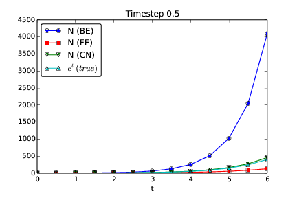
Reducing the time step to 0.05, it changes into:

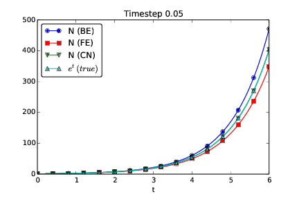
We observe that CN produces the best solution of the three alternatives. This should be expected, since it is the most accurate one (second order accuracy compared to first order with FE and BE).

Filename: growth_CN.m.

Exercise 55: Understand finite differences via Taylor series

The Taylor series around a point \(x=a\) can for a function \(f(x)\) be written

\[\begin{split}f(x) &= f(a) + \frac{d}{dx}f(a)(x-a) + \frac{1}{2!}\frac{d^2}{dx^2}f(a)(x-a)^2 \\ &\quad + \frac{1}{3!}\frac{d^3}{dx^3}f(a)(x-a)^3 + \ldots\\ & = \sum_{i=0}^\infty \frac{1}{i!}\frac{d^i}{dx^i}f(a)(x-a)^i\thinspace .\end{split}\]

For a function of time, as addressed in our ODE problems, we would use \(u\) instead of \(f\), \(t\) instead of \(x\), and a time point \(t_n\) instead of \(a\):

\[\begin{split}u(t) &= u(t_n) + \frac{d}{dt}u(t_n)(t-t_n) + \frac{1}{2!}\frac{d^2}{dt^2}u(t_n)(t-t_n)^2\\ &\quad + \frac{1}{3!}\frac{d^3}{dt^3}u(t_n)(t-t_n)^3 + \ldots\\ & = \sum_{i=0}^\infty \frac{1}{i!}\frac{d^i}{dt^i}u(t_n)(t-t_n)^i\thinspace .\end{split}\]

a) A forward finite difference approximation to the derivative \(f'(a)\) reads

\[u'(t_n) \approx \frac{u(t_n+\Delta t)- u(t_n)}{\Delta t}\thinspace .\]

We can justify this formula mathematically through Taylor series. Write up the Taylor series for \(u(t_n+\Delta t)\) (around \(t=t_n\), as given above), and then solve the expression with respect to \(u'(t_n)\). Identify, on the right-hand side, the finite difference approximation and an infinite series. This series is then the error in the finite difference approximation. If \(\Delta t\) is assumed small (i.e. \(\Delta t << 1\)), \(\Delta t\) will be much larger than \(\Delta t^2\), which will be much larger than \(\Delta t^3\), and so on. The leading order term in the series for the error, i.e., the error with the least power of \(\Delta t\) is a good approximation of the error. Identify this term.

Solution. We get

\[\begin{split}u(t_n+\Delta t) &= u(t_n) + \frac{d}{dt}u(t_n)\Delta t + \frac{1}{2!}\frac{d^2}{dt^2}u(t_n)\Delta t^2 + \frac{1}{3!}\frac{d^3}{dt^3}u(t_n)\Delta t^3 + \ldots\\ \frac{d}{dt}u(t_n) & = \frac{u(t_n+\Delta t) - u(t_n)}{\Delta t} - \frac{1}{2!}\frac{d^2}{dt^2}u(t_n)\Delta t - \frac{1}{3!}\frac{d^3}{dt^3}u(t_n)\Delta t^2 + \ldots\\ \thinspace .\end{split}\]

The finite difference approximation is found as the first term on the right hand side, while the remaining terms make up the infinite series that represents the error of the finite difference approximation.

The leading order error term is therefore \(-\frac{1}{2!}\frac{d^2}{dt^2}u(t_n)\Delta t\).

b) Repeat a) for a backward difference:

\[u'(t_n) \approx \frac{u(t_n)- u(t_n-\Delta t)}{\Delta t}\thinspace .\]

This time, write up the Taylor series for \(u(t_n-\Delta t)\) around \(t_n\). Solve with respect to \(u'(t_n)\), and identify the leading order term in the error. How is the error compared to the forward difference?

Solution. We get

\[\begin{split}u(t_n-\Delta t) &= u(t_n) - \frac{d}{dt}u(t_n)\Delta t + \frac{1}{2!}\frac{d^2}{dt^2}u(t_n)\Delta t^2 - \frac{1}{3!}\frac{d^3}{dt^3}u(t_n)\Delta t^3 + \ldots\\ \frac{d}{dt}u(t_n) & = \frac{u(t_n) - u(t_n-\Delta t)}{\Delta t} + \frac{1}{2!}\frac{d^2}{dt^2}u(t_n)\Delta t - \frac{1}{3!}\frac{d^3}{dt^3}u(t_n)\Delta t^2 + \ldots\\ \thinspace .\end{split}\]

The finite difference approximation is found as the first term on the right hand side, while the remaining terms make up the infinite series that represents the error of the finite difference approximation.

The leading order error term is therefore \(+\frac{1}{2!}\frac{d^2}{dt^2}u(t_n)\Delta t\), which is of the same magnitude as the corresponding error in a), but with opposite sign.

c) A centered difference approximation to the derivative, as explored in Exercise 54: Use a Crank-Nicolson scheme for population growth, can be written

\[u'(t_n+\frac{1}{2}\Delta t) \approx \frac{u(t_n+\Delta t)- u(t_n)}{\Delta t}\thinspace .\]

Write up the Taylor series for \(u(t_n)\) around \(t_n+\frac{1}{2}\Delta t\) and the Taylor series for \(u(t_n+\Delta t)\) around \(t_n+\frac{1}{2}\Delta t\). Subtract the two series, solve with respect to \(u'(t_n+\frac{1}{2}\Delta t)\), identify the finite difference approximation and the error terms on the right-hand side, and write up the leading order error term. How is this term compared to the ones for the forward and backward differences?

Solution. We write

\[\begin{split}u(t_n) &= u(t_n+\frac{\Delta t}{2}) - \frac{d}{dt}u(t_n+\frac{\Delta t}{2})\frac{\Delta t}{2} + \frac{1}{2!}\frac{d^2}{dt^2}u(t_n+\frac{\Delta t}{2})\left(\frac{\Delta t}{2}\right)^2\\ &\quad - \frac{1}{3!}\frac{d^3}{dt^3}u(t_n+\frac{\Delta t}{2})\left(\frac{\Delta t}{2}\right)^3 + \ldots\\ u(t_n+\Delta t) &= u(t_n+\frac{\Delta t}{2}) + \frac{d}{dt}u(t_n+\frac{\Delta t}{2})\frac{\Delta t}{2} + \frac{1}{2!}\frac{d^2}{dt^2}u(t_n+\frac{\Delta t}{2})\left(\frac{\Delta t}{2}\right)^2\\ &\quad + \frac{1}{3!}\frac{d^3}{dt^3}u(t_n+\frac{\Delta t}{2})\left(\frac{\Delta t}{2}\right)^3 + \ldots\\ \thinspace .\end{split}\]

If we next subtract the first of these two equations from the last one, we may proceed as

\[\begin{split}u(t_n+\Delta t) - u(t_n) &= 2\frac{d}{dt}u(t_n+\frac{\Delta t}{2})\frac{\Delta t}{2} + 2\frac{1}{3!}\frac{d^3}{dt^3}u(t_n+\frac{\Delta t}{2})\left(\frac{\Delta t}{2}\right)^3 + \ldots\\ \frac{d}{dt}u(t_n+\frac{\Delta t}{2}) &= \frac{u(t_n+\Delta t) - u(t_n)}{\Delta t} - \frac{1}{3!}\frac{d^3}{dt^3}u(t_n+\frac{\Delta t}{2})\left(\frac{\Delta t}{2}\right)^2 - \ldots\\ \thinspace .\end{split}\]

The finite difference approximation is found as the first term on the right hand side, while the remaining terms make up the infinite series that represents the error of the finite difference approximation.

The leading order error term is \(-\frac{1}{3!}\frac{d^3}{dt^3}u(t_n+\frac{\Delta t}{2})\left(\frac{\Delta t}{2}\right)^2\). This term will be smaller than the corresponding error terms from the previous approximations since \(\frac{\Delta t}{2}^2 << \Delta t\).

d) Can you use the leading order error terms in a)-c) to explain the visual observations in the numerical experiment in Exercise 54: Use a Crank-Nicolson scheme for population growth?

Solution. The error term for the centered difference is \(\Delta t^2\) and hence smaller than the error terms for the forward and backward differences. Therefore, the Crank-Nicolson curve is closer to the analytical solution. Also, the error terms of the forward and backward differences are the same, except for the sign, which explains why the corresponding curves lie on each side of the analytical solution, with approximately the same distance. Note: the leading order error term is only a good approximation to the true error as \(\Delta t\rightarrow 0\), so for small \(\Delta t\), the forward and backward schemes will deviate an equal amount from the analytical solution in the center, but for large \(\Delta t\) errors will deviate from this observation (and, in particular, the backward scheme may give oscillatory solutions for large \(\Delta t\) in this problem).

e) Find the leading order error term in the following standard finite difference approximation to the second-order derivative:

\[u''(t_n) \approx \frac{u(t_n+\Delta t)- 2u(t_n) + u(t_n-\Delta t)}{\Delta t}\thinspace .\]

Hint. Express \(u(t_n\pm \Delta t)\) via Taylor series and insert them in the difference formula.

Solution. We write

\[\begin{split}u(t_n+\Delta t) &= u(t_n) + \frac{d}{dt}u(t_n)\Delta t + \frac{1}{2!}\frac{d^2}{dt^2}u(t_n)\Delta t^2 + \frac{1}{3!}\frac{d^3}{dt^3}u(t_n)\Delta t^3 + \ldots\\ u(t_n-\Delta t) &= u(t_n) - \frac{d}{dt}u(t_n)\Delta t + \frac{1}{2!}\frac{d^2}{dt^2}u(t_n)\Delta t^2 - \frac{1}{3!}\frac{d^3}{dt^3}u(t_n)\Delta t^3 + \ldots\\ \thinspace .\end{split}\]

If we now add the two equations, it gives us

\[u(t_n+\Delta t) + u(t_n-\Delta t) = 2 u(t_n) + 2\frac{1}{2!}\frac{d^2}{dt^2}u(t_n)\Delta t^2 + 2\frac{1}{4!}\frac{d^4}{dt^4}u(t_n)\Delta t^4 + \ldots\thinspace .\]

This allows us to isolate \(u''(t_n)\) on the left hand side as

\[\frac{d^2}{dt^2}u(t_n) = \frac{u(t_n+\Delta t) - 2 u(t_n) + u(t_n-\Delta t)}{\Delta t^2} - 2\frac{1}{4!}\frac{d^4}{dt^4}u(t_n)\Delta t^2 - \ldots\thinspace .\]

The leading error term therefore appears as \(-2\frac{1}{4!}\frac{d^4}{dt^4}u(t_n)\Delta t^2\).

Filename: Taylor_differences.pdf.

Exercise 56: Use a Backward Euler scheme for oscillations

Consider (71)-(72) modeling an oscillating engineering system. This \(2\times 2\) ODE system can be solved by the Backward Euler scheme, which is based on discretizing derivatives by collecting information backward in time. More specifically, \(u'(t)\) is approximated as

\[u'(t) \approx \frac{u(t) - u(t-\Delta t)}{\Delta t}\thinspace .\]

A general vector ODE \(u'=f(u,t)\), where \(u\) and \(f\) are vectors, can use this approximation as follows:

\[\frac{u^{n} - u^{n-1}}{\Delta t} = f(u^n,t_n),\]

which leads to an equation for the new value \(u^n\):

\[u^n -\Delta tf(u^n,t_n) = u^{n-1}\thinspace .\]

For a general \(f\), this is a system of nonlinear algebraic equations.

However, the ODE (71)-(72) is linear, so a Backward Euler scheme leads to a system of two algebraic equations for two unknowns:

\[\tag{114} u^{n} - \Delta t v^{n} = u^{n-1},\]

\[\tag{115} v^{n} + \Delta t \omega^2 u^{n} = v^{n-1}\]\[ \thinspace .\]

a) Solve the system for \(u^n\) and \(v^n\).

Solution. In the first of these equations, we may isolate \(u^n\) on the left hand side. This gives

\[u^n = \Delta t v^n + u^{n-1}\thinspace .\]

Inserting this for \(u^n\) in the second equation, we can solve for \(v^n\). That is,

\[v^n + \Delta t \omega^2 (\Delta t v^n + u^{n-1}) = v^{n-1}\thinspace ,\]

so that

\[v^n = \frac{1}{1 + (\Delta t \omega)^2}(-\Delta t \omega^2 u^{n-1} + v^{n-1})\thinspace .\]

Finally, we may insert this expression for \(v^n\) into the one for \(u^n\), which gives

\[u^n = \Delta t (\frac{1}{1 + (\Delta t \omega)^2}(-\Delta t \omega^2 u^{n-1} + v^{n-1})) + u^{n-1}\thinspace .\]

Simplifying, we arrive at

\[u^n = \frac{\Delta t v^{n-1} + u^{n-1}}{1 + (\Delta t \omega)^2}\thinspace .\]

Thus, we have an explicit scheme for advancing the solution \(v^n\) and \(u^n\) in time.

b) Implement the found formulas for \(u^n\) and \(v^n\) in a program for computing the entire numerical solution of (71)-(72).

Solution.

omega = 2;
P = 2*pi/omega;
dt = P/20;
%dt = P/2000;
T = 3*P;
N_t = floor(round(T/dt));
t = linspace(0, N_t*dt, N_t+1);

u = zeros(N_t+1, 1);
v = zeros(N_t+1, 1);

% Initial condition
X_0 = 2;
u(1) = X_0;
v(1) = 0;

% Step equations forward in time
for n = 2:N_t+1
    u(n) = (1.0/(1+(dt*omega)^2)) * (dt*v(n-1) + u(n-1));
    v(n) = (1.0/(1+(dt*omega)^2)) * (-dt*omega^2*u(n-1) + v(n-1));
end

plot(t, u, 'b-', t, X_0*cos(omega*t), 'r--');
legend('numerical', 'exact', 'Location', 'northwest');
xlabel('t');
print('tmp', '-dpdf');  print('tmp', '-dpng');

c) Run the program with a \(\Delta t\) corresponding to 20 time steps per period of the oscillations (see the section Programming the numerical method; the special case for how to find such a \(\Delta t\)). What do you observe? Increase to 2000 time steps per period. How much does this improve the solution?

Solution. With 20 time steps per period, the oscillations develop as

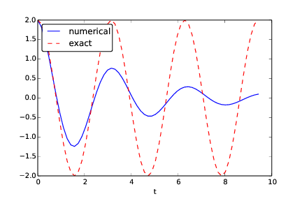
Changing to 2000 time steps per period, the solution improves dramatically into

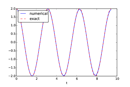
Filename: osc_BE.m.

Remarks

While the Forward Euler method applied to oscillation problems \(u''+\omega^2u=0\) gives growing amplitudes, the Backward Euler method leads to significantly damped amplitudes.

Exercise 57: Use Heun’s method for the SIR model

Make a program that computes the solution of the SIR model from the section Spreading of a flu both by the Forward Euler method and by Heun’s method (or equivalently: the 2nd-order Runge-Kutta method) from the section The 2nd-order Runge-Kutta method (or Heun’s method). Compare the two methods in the simulation case from the section Programming the numerical method; the special case. Make two comparison plots, one for a large and one for a small time step. Experiment to find what “large” and “small” should be: the large one gives significant differences, while the small one lead to very similar curves.

Solution.

% Time unit: 1 h
beta = 10.0/(40*8*24);
gamma = 3.0/(15*24);
%dt = 4.0;            % Small dt
dt = 24.0;            % Large dt
D = 30;               % Simulate for D days
N_t = floor(D*24/dt); % Corresponding no of hours

t = linspace(0, N_t*dt, N_t+1);
S_FE = zeros(N_t+1, 1);
I_FE = zeros(N_t+1, 1);
R_FE = zeros(N_t+1, 1);
S_H  = zeros(N_t+1, 1);
I_H  = zeros(N_t+1, 1);
R_H  = zeros(N_t+1, 1);

% Initial condition
S_FE(1) = 50; I_FE(1) = 1; R_FE(1) = 0;
S_H(1) = 50;  I_H(1) = 1;  R_H(1) = 0;

% Step equations forward in time
for n = 1:N_t
    % FE
    S_FE(n+1) = S_FE(n) - dt*beta*S_FE(n)*I_FE(n);
    I_FE(n+1) = I_FE(n) + dt*beta*S_FE(n)*I_FE(n) - dt*gamma*I_FE(n);
    R_FE(n+1) = R_FE(n) + dt*gamma*I_FE(n);
    % H  (predict and then update)
    S_p = S_H(n) - dt*beta*S_H(n)*I_H(n);
    I_p = I_H(n) + dt*beta*S_H(n)*I_H(n) - dt*gamma*I_H(n);
    R_p = R_H(n) + dt*gamma*I_H(n);

    S_H(n+1) = S_H(n) - (dt/2.0)*(beta*S_H(n)*I_H(n) +...
                                              beta*S_p*I_p);
    I_H(n+1) = I_H(n) +...
               (dt/2.0)*(beta*S_H(n)*I_H(n) - gamma*I_H(n) +...
                         beta*S_p*I_p - gamma*I_p);
    R_H(n+1) = R_H(n) + (dt/2.0)*(gamma*I_H(n) + gamma*I_p );
end

plot(t, S_FE, t, I_FE, t, R_FE, t, S_H, t, I_H, t, R_H);
legend('S (FE)', 'I (FE)', 'R (FE)', 'S (H)', 'I (H)', 'R (H)',...
                             'Location', 'northwest');
xlabel('hours');
print('tmp', '-dpdf');  print('tmp', '-dpng');

With a (large) time step of \(24 h\), we get the following behavior,

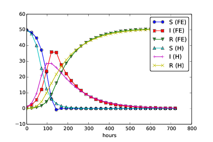
Reducing the time step to \(4 h\), the curves get very similar.

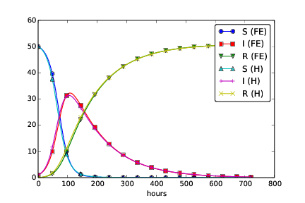
Filename: SIR_Heun.m.

Exercise 58: Use Odespy to solve a simple ODE

Solve

\[u' = -au + b,\quad u(0)=U_0,\quad t\in (0,T]\]

by the Odespy software. Let the problem parameters \(a\) and \(b\) be arguments to the right-hand side function that specifies the ODE to be solved. Plot the solution for the case when \(a=2\), \(b=1\), \(T=6/a\), and we use 100 time intervals in \([0,T]\).

Solution.

import odespy
import numpy as np
import matplotlib.pyplot as plt

def f(u, t, a, b):
    return -a*u + b

# Problem parameters
a = 2
b = 1
U0 = 2
method = odespy.RK2

# Run Odespy solver
solver = method(f, f_args=[a, b])
solver.set_initial_condition(U0)
T = 6.0/a  # final simulation time
N_t = 100  # no of intervals
time_points = np.linspace(0, T, N_t+1)
u, t = solver.solve(time_points)

plt.plot(t, u)
plt.show

Filename: odespy_demo.m.

Exercise 59: Set up a Backward Euler scheme for oscillations

Write the ODE \(u'' + \omega^2u=0\) as a system of two first-order ODEs and discretize these with backward differences as illustrated in Figure Illustration of a backward difference approximation to the derivative. The resulting method is referred to as a Backward Euler scheme. Identify the matrix and right-hand side of the linear system that has to be solved at each time level. Implement the method, either from scratch yourself or using Odespy (the name is odespy.BackwardEuler). Demonstrate that contrary to a Forward Euler scheme, the Backward Euler scheme leads to significant non-physical damping. The figure below shows that even with 60 time steps per period, the results after a few periods are useless:

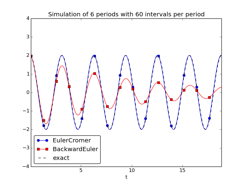
Solution. The first-order system is

\[\begin{split}v' &= -\omega^2 u\\ u' &= v\end{split}\]

Backward differences mean

\[\begin{split}\frac{v^{n}-v^{n-1}}{\Delta t} &= -\omega^2 u^n\\ \frac{u^{n}-u^{n-1}}{\Delta t} &= v^n\end{split}\]

Collecting the unknowns \(u^n\) and \(v^n\) on the left-hand side,

\[\begin{split}v^{n} + \Delta t\omega^2 u^n &= v^{n-1} \\ u^{n} - \Delta t v^n &= u^{n-1}\end{split}\]

shows that this is a coupled \(2\times 2\) system for \(u^n\) and \(v^n\):

\[\begin{split}\left(\begin{array}{cc} 1 & \Delta t\omega^2\\ -\Delta t & 1 \end{array}\right) \left(\begin{array}{c} v^n\\ u^n \end{array}\right) = \left(\begin{array}{c} v^{n-1}\\ u^{n-1} \end{array}\right)\end{split}\]

The simplest way of implementing the scheme is to use the osc_odespy.py code explained in the section Software for solving ODEs and make a call

compare(odespy_methods=[odespy.EulerCromer, odespy.BackwardEuler],
        omega=2, X_0=2,number_of_periods=6,
        time_intervals_per_period=60)

Filename: osc_BE.m.

Exercise 60: Set up a Forward Euler scheme for nonlinear and damped oscillations

Derive a Forward Euler method for the ODE system (96)-(97). Compare the method with the Euler-Cromer scheme for the sliding friction problem from the section Spring-mass system with sliding friction:

1. Does the Forward Euler scheme give growing amplitudes?
2. Is the period of oscillation accurate?
3. What is the required time step size for the two methods to have visually coinciding curves?

Solution. A Forward Euler scheme is easy to derive:

\[\tag{116} \frac{v^{n+1}-v^n}{\Delta t} = \frac{1}{m}\left(F(t_n) - s(u^n) - f(v^n)\right),\]

\[\tag{117} \frac{u^{n+1}-u^n}{\Delta t} = v^n,\]

which is, as usual, reordered to the algorithmic form

\[\tag{118} v^{n+1} = v^n + \frac{\Delta t}{m}\left(F(t_n) - s(u^n) - f(v^n)\right),\]

\[\tag{119} u^{n+1} = u^n + \Delta t v^n\thinspace .\]

However, we have already seen that the Forward Euler method is not well suited for simulating oscillations as the scheme gives rise to a non-physical, growing amplitude. It remains to see how damped systems are treated.

An implementation can be done utilizing Odespy and the compare function in osc_odespy_general.py:

def sliding_friction():
    from numpy import tanh, sign

    f = lambda v: mu*m*g*sign(v)
    alpha = 60.0
    s = lambda u: k/alpha*tanh(alpha*u)
    #s = lambda u: k*u
    F = lambda t: 0

    g = 9.81
    mu = 0.4
    m = 1
    k = 1000

    U_0 = 0.1
    V_0 = 0

    T = 1
    dt = T/100.

    methods = [odespy.EulerCromer, odespy.ForwardEuler]
    compare(methods, f=f, s=s, F=F, m=1, U_0=U_0, V_0=V_0,
            T=T, dt=dt, start_of_plot=0)

With \(\Delta t =10^{-2}\) we get the plot below.

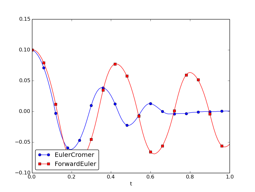
We observe that 1) the amplitude is not growing, it is decaying, but not at all at the rate it should, compared to the Euler-Cromer scheme (which we anticipate is fairly accurate, also for this fairly coarse time resolution), and 2) there is a significant phase error.

Reducing \(\Delta t\) by a factor of 10 increases the accuracy incredibly:

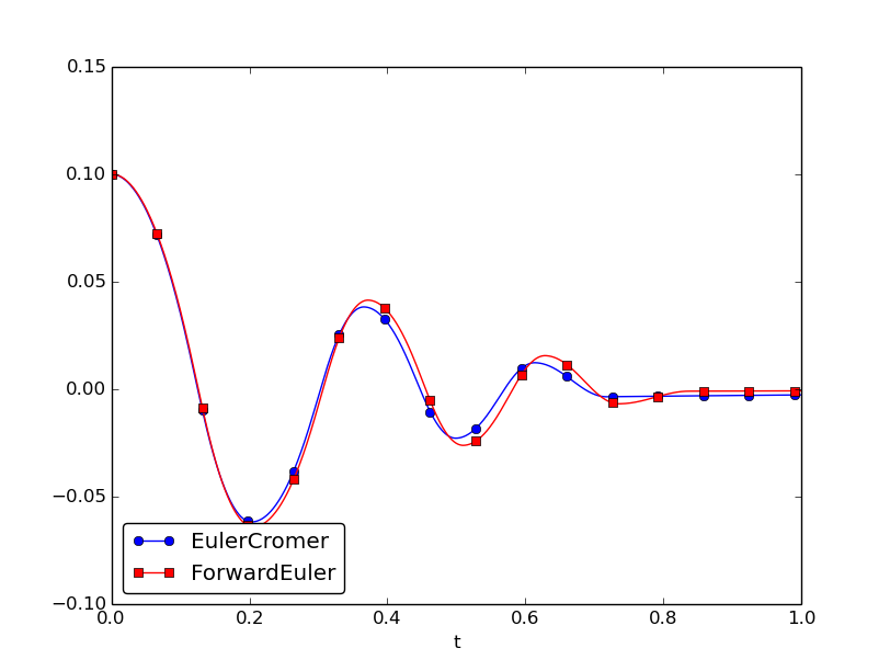
Experimenting a bit, we arrive at \(\Delta t=5\cdot 10^{-3}\) as a time step size where the two methods gives approximately equal results:

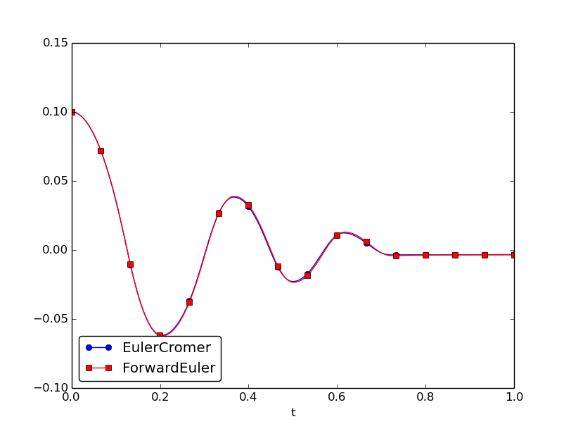
Filename: osc_FE_general.m.

Exercise 61: Discretize an initial condition

Assume that the initial condition on \(u'\) is nonzero in the finite difference method from the section A finite difference method; undamped, linear case: \(u'(0)=V_0\). Derive the special formula for \(u^1\) in this case.

Solution. We use the same centered finite difference approximation,

\[u'(0)\approx = \frac{u^1 - u^{-1}}{2\Delta t}=V_0,\]

which leads to

\[u^{-1} = u^1 - 2\Delta t\,V_0\thinspace .\]

Using this expression to eliminate \(u^{-1}\) in (105) leads to

\[u^1 = u^0 + \Delta t\,V_0 - \frac{1}{2}\Delta t^2\omega^2 u^0\thinspace .\]

Filename: ic_with_V_0.pdf.