This chapter is taken from the book A Primer on Scientific Programming with Python by H. P. Langtangen, 5th edition, Springer, 2016.
Class hierarchy for numerical differentiation
The document Introduction to classes in
Python [2]
presents a class Derivative that (approximately) differentiate any
mathematical function represented by a callable Python object. The
class employs the simplest possible numerical derivative. There are a
lot of other numerical formulas for computing approximations to
\( f'(x) \):
$$
\begin{align}
f'(x) &= \frac{f(x+h)-f(x)}{h} + \mathcal{O}(h),
\quad\hbox{(1st-order forward diff.)}
\tag{1}\\
f'(x) &= \frac{f(x)-f(x-h)}{h} + \mathcal{O}(h),
\quad\hbox{(1st-order backward diff.)}
\tag{2}\\
f'(x) &= \frac{f(x+h)-f(x-h)}{2h} + \mathcal{O}(h^2),
\quad\hbox{(2nd-order central diff.)}
\tag{3}\\
f'(x) &= \frac{4}{3}\frac{f(x+h)-f(x-h)}{2h}
-\frac{1}{3}\frac{f(x+2h) - f(x-2h)}{4h} + \mathcal{O}(h^4),
\nonumber\\
& \quad\hbox{(4th-order central diff.)} \tag{4}\\
f'(x) &= \frac{3}{2}\frac{f(x+h)-f(x-h)}{2h}
-\frac{3}{5}\frac{f(x+2h) - f(x-2h)}{4h} + \nonumber\\
& \frac{1}{10}\frac{f(x+3h) - f(x-3h)}{6h} + \mathcal{O}(h^6),\nonumber\\
& \quad\hbox{(6th-order central diff.)}
\tag{5}\\
f'(x) &= \frac{1}{h}\left(
-\frac{1}{6}f(x+2h) + f(x+h) - \frac{1}{2}f(x) - \frac{1}{3}f(x-h)\right)
+ \mathcal{O}(h^3),\nonumber\\
& \quad\hbox{(3rd-order forward diff.)}
\tag{6}
\end{align}
$$
The key ideas about the implementation of such a family of formulas
are explained in the section Classes for differentiation. For the interested reader,
the sections Extensions-Alternative implementation via a single class contains
more advanced additional material that can well be skipped in a first
reading. However, the additional material puts the basic solution in
the section Classes for differentiation into a wider perspective, which may increase
the understanding of object orientation.
Classes for differentiation
It is argued in the document Introduction to classes in
Python [2]
that it is wise to implement a numerical differentiation formula as a
class where \( f(x) \) and \( h \) are data attributes and a __call__ method
makes class instances behave as ordinary Python functions. Hence,
when we have a collection of different numerical differentiation
formulas, like (1)-(6), it makes sense
to implement each one of them as a class.
Doing this implementation
we realize that the constructors are identical because their task in
the present case to store \( f \) and \( h \). Object-orientation is now a
natural next step: we can avoid duplicating the constructors by
letting all the classes inherit the common constructor code. To this
end, we introduce a superclass Diff and implement the different
numerical differentiation rules in subclasses of Diff. Since the
subclasses inherit their constructor, all they have to do is to
provide a __call__ method that implements the relevant
differentiation formula.
Let us show what the superclass Diff looks like and how
three subclasses implement the
formulas (1)-(3):
class Diff(object):
    def __init__(self, f, h=1E-5):
        self.f = f
        self.h = float(h)

class Forward1(Diff):
    def __call__(self, x):
        f, h = self.f, self.h
        return (f(x+h) - f(x))/h

class Backward1(Diff):
    def __call__(self, x):
        f, h = self.f, self.h
        return (f(x) - f(x-h))/h

class Central2(Diff):
    def __call__(self, x):
        f, h = self.f, self.h
        return (f(x+h) - f(x-h))/(2*h)
These small classes demonstrates an important feature of object-orientation: code common to many different classes are placed in a superclass, and the subclasses add just the code that differs among the classes.
We can easily implement the formulas (4)-(6) by following the same method:
class Central4(Diff):
    def __call__(self, x):
        f, h = self.f, self.h
        return (4./3)*(f(x+h)   - f(x-h))  /(2*h) - \
               (1./3)*(f(x+2*h) - f(x-2*h))/(4*h)

class Central6(Diff):
    def __call__(self, x):
        f, h = self.f, self.h
        return (3./2) *(f(x+h)   - f(x-h))  /(2*h) - \
               (3./5) *(f(x+2*h) - f(x-2*h))/(4*h) + \
               (1./10)*(f(x+3*h) - f(x-3*h))/(6*h)

class Forward3(Diff):
    def __call__(self, x):
        f, h = self.f, self.h
        return (-(1./6)*f(x+2*h) + f(x+h) - 0.5*f(x) - \
                (1./3)*f(x-h))/h
We have placed all the classes in a module file Diff.py. Here is a short interactive example using the module to numerically differentiate the sine function:
>>> from Diff import *
>>> from math import sin
>>> mycos = Central4(sin)
>>> mycos(pi)              # compute sin'(pi)
-1.000000082740371
Instead of a plain Python function we may use an object with a
__call__ method, here exemplified through the
function \( f(t;a,b,c)=at^2 + bt + c \):
class Poly2(object):
    def __init__(self, a, b, c):
        self.a, self.b, self.c = a, b, c
    def __call__(self, t):
        return self.a*t**2 + self.b*t + self.c

f = Poly2(1, 0, 1)
dfdt = Central4(f)
t = 2
print "f'(%g)=%g" % (t, dfdt(t))
Let us examine the program flow.
When Python encounters dfdt = Central4(f),
it looks for the constructor in class Central4, but there is no
constructor in that class. Python then examines the superclasses
of Central4, listed in Central4.__bases__.
The superclass Diff contains a constructor, and this method
is called. When Python meets the dfdt(t) call, it looks
for __call__ in class Central4 and finds it, so there
is no need to examine the superclass. This process of looking up
methods of a class is called dynamic binding.
Computer science remark
Dynamic binding means that a name is bound to a function while the program is running. Normally, in computer languages, a function name is static in the sense that it is hardcoded as part of the function body and will not change during the execution of the program. This principle is known as static binding of function/method names. Object orientation offers the technical means to associate different functions with the same name, which yields a kind of magic for increased flexibility in programs. The particular function that the name refers to can be set at run-time, i.e., when the program is running, and therefore known as dynamic binding.
In Python, dynamic binding is a natural feature since names
(variables) can refer to functions and therefore be dynamically bound
during execution, just as any ordinary variable. To illustrate this
point, let func1 and func2 be two Python functions of one
argument, and consider the code
if input == 'func1':
    f = func1
elif input == 'func2':
    f = func2
y = f(x)
Here, the name f is bound to one of the func1 and func2 function
objects while the program is running. This is a result of two
features: (i) dynamic typing (so the contents of f can change), and
(ii) functions being ordinary objects. The bottom line is that
dynamic binding comes natural in Python, while it appears more like
convenient magic in languages like C++, Java, and C#.
Verification
We have several alternative numerical methods for differentiation
implemented in the Diff hierarchy, and the Diff module should
contain one or more test functions for verifying the
implementations. The fundamental problem is that even if we know the
exact derivative of a function, we do not know what the numerical
error in one of the subclass methods is. This fact prevents us from
comparing the numerical and the exact derivative.
Fortunately, numerical differentiation formulas of the type we have encountered above are able to differentiate lower order polynomials exactly. All of them are capable of computing \( f'(x)=a \), where \( f(x)=ax+b \), without approximation errors for any \( h \). We can use this knowledge to construct a test function:
def test_Central2():
    def f(x):
        return a*x + b

    def df_exact(x):
        return a

    a = 0.2; b = -4
    df = Central2(f, h=0.55)
    x = 6.2
    msg = 'method Central2 failed: df/dx=%g != %g' % \
          (df(x), df_exact(x))
    tol = 1E-14
    assert abs(df_exact(x) - df(x)) < tol
It will be boring to write such a test function for each class
in the hierarchy. Therefore, we parameterize the class name
and rewrite test_Central such that it can be reused for
any class in the Diff hierarchy:
def _test_one_method(method):
    """Test method in string `method` on a linear function."""
    f = lambda x: a*x + b
    df_exact = lambda x: a
    a = 0.2; b = -4
    df = eval(method)(f, h=0.55)
    x = 6.2
    msg = 'method %s failed: df/dx=%g != %g' % \
          (method, df(x), df_exact(x))
    tol = 1E-14
    assert abs(df_exact(x) - df(x)) < tol
Some comments are needed to explain this function:
- All our test functions are intended for the pytest and nose testing
frameworks.
(See The
document Unit testing with pytest and nose
[3] for more information on such test functions.)
The function name must then start with
test_and no arguments are allowed. For the helper function_test_one_methodwith an argument, the function name cannot start withtest, and that is why an underscore is added. - Lambda functions
are used to save code in the definitions of
fanddf_exact. - The subclass to be tested is given as a string
method. Calling the constructor must then be done byeval(method)(f).
_test_one_method for each of them. As always, we try to find
a way to automate boring work, which here consists of listing all
the subclasses (and remembering to update the list when new subclasses
are added). All global variables in a file is available from the
dictionary returned by globals(). The key is a variable name and
the value is the corresponding object. For example, print globals()
reveals that all the defined classes are in globals(), e.g.,
'Central2': <class Diff.Central2 at 0x1a87c80>,
'Central4': <class Diff.Central4 at 0x1a87f58>,
'Diff': <class Diff.Diff at 0x1a870b8>,
To find all the relevant classes to test, we grab all names from
the globals() dictionary, look for names that starts with upper case,
and find the names that correspond to a subclass of Diff (drop Diff
itself as this class cannot compute anything and therefore cannot be
tested). Translating this algorithm to code gives us a test function
that can test all subclasses in the Diff hierarchy:
def test_all_methods():
    """Call _test_one_method for all subclasses of Diff."""
    print globals()
    names = list(globals().keys())  # all names in this module
    for name in names:
        if name[0].isupper():
            if issubclass(eval(name), Diff):
                if name != 'Diff':
                    _test_one_method(name)
A flexible main program
As a demonstration of the power of Python programming, we shall now
write a main program for our Diff module
that accepts a function on the command-line, together with
information about the difference type (centered, backward, or forward),
the order of the approximation, and a value of the independent variable.
The corresponding output is the derivative of the given function.
An example of the usage of the program goes like this:
Diff.py 'exp(sin(x))' Central 2 3.1
-1.04155573055
Here, we asked the program to differentiate \( f(x)=e^{\sin x} \)
at \( x=3.1 \) with a central scheme of order 2 (using the Central2 class
in the Diff hierarchy).
We can provide any expression with x as input and request any
scheme from the Diff hierarchy, and the derivative will be
(approximately) computed. One great thing with Python is that the
code is very short:
from math import *  # make all math functions available to main

def main():
    from scitools.StringFunction import StringFunction
    import sys

    try:
        formula = sys.argv[1]
        difftype = sys.argv[2]
        difforder = sys.argv[3]
        x = float(sys.argv[4])
    except IndexError:
        print 'Usage:   Diff.py formula difftype difforder x'
        print 'Example: Diff.py "sin(x)*exp(-x)" Central 4 3.14'
        sys.exit(1)

    classname = difftype + difforder
    f = StringFunction(formula)
    df = eval(classname)(f)
    print df(x)

if __name__ == '__main__':
    main()
Read the code line by line, and convince yourself that you understand
what is going on.
You may need to review the eval function and the StringFunction tool (see
pydoc scitools.StringFunction.StringFunction).
One disadvantage is that the code above is limited to x as the name
of the independent variable. If we allow a 5th command-line argument
with the name of the independent variable, we can pass this name on
to the StringFunction constructor, and suddenly our program
works with any name for the independent variable!
varname = sys.argv[5]
f = StringFunction(formula, independent_variables=varname)
Of course, the program crashes if we do not provide five command-line arguments, and the program does not work properly if we are not careful with ordering of the command-line arguments. There is some way to go before the program is really user friendly, but that is beyond the scope of this document.
Many other popular programming languages (C++, Java, C#) cannot
perform the eval operation while the program is running.
The result is that one needs if tests to turn the information
in difftype and difforder
into creation of subclass instances. Such type of code
would look like this in Python:
if classname == 'Forward1':
    df = Forward1(f)
elif classname == 'Backward1':
    df = Backward1(f)
...
and so forth. This piece of code is very common in object-oriented
systems and often put in a function that is referred to as a
factory function.
Thanks to eval in Python, factory functions are usually only a matter of
applying eval to a string.
Extensions
The great advantage of sharing code via inheritance becomes obvious
when we want to extend the functionality of a class hierarchy. It is
possible to do this by adding more code to the superclass only.
Suppose we want to be able to assess the accuracy of the numerical
approximation to the derivative by comparing with the exact
derivative, if available. All we need to do is to allow an extra
argument in the constructor and provide an additional superclass
method that computes the error in the numerical derivative. We may
add this code to class Diff, or we may add it in a subclass Diff2
and let the other classes for various numerical differentiation
formulas inherit from class Diff2. We follow the latter approach:
class Diff2(Diff):
    def __init__(self, f, h=1E-5, dfdx_exact=None):
        Diff.__init__(self, f, h)
        self.exact = dfdx_exact

    def error(self, x):
        if self.exact is not None:
            df_numerical = self(x)
            df_exact = self.exact(x)
            return df_exact - df_numerical

class Forward1(Diff2):
    def __call__(self, x):
        f, h = self.f, self.h
        return (f(x+h) - f(x))/h
The other subclasses, Backward1, Central2, and so on, must
also be derived from Diff2 to equip all subclasses with new
functionality for perfectly assessing the accuracy of the approximation.
No other modifications are necessary in this example, since all the
subclasses can inherit the superclass constructor and the error
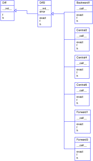
method. Figure 2 shows a UML diagram of
the new Diff class hierarchy.
Figure 2: UML diagram of the Diff hierarchy for a series of differentiation formulas (Backward1, Central2, etc.).
Here is an example of usage:
mycos = Forward1(sin, dfdx_exact=cos)
print 'Error in derivative is', mycos.error(x=pi)
The program flow of the mycos.error(x=pi)
call can be interesting to follow.
We first enter the error method in class Diff2,
which then calls self(x), i.e., the __call__ method
in class Forward1, which jumps out to the self.f function,
i.e., the sin function in the math module in the present case.
After returning to the error method,
the next call is to self.exact, which is the cos function
(from math) in our case.
Application
We can apply the methods in the Diff2 hierarchy to get some insight
into the accuracy of various difference formulas. Let us write out a
table where the rows correspond to different \( h \) values, and the
columns correspond to different approximation methods (except the
first column, which reflects the \( h \) value). The values in the table
can be the numerically computed \( f'(x) \) or the error in this
approximation if the exact derivative is known. The following function
writes such a table:
def table(f, x, h_values, methods, dfdx=None):
    # Print headline (h and class names for the methods)
    print '      h       ',
    for method in methods:
        print '%-15s' % method.__name__,
    print  # newline
    # Print table
    for h in h_values:
        print '%10.2E' % h,
        for method in methods:
            if dfdx is not None:       # write error
                d = method(f, h, dfdx)
                output = d.error(x)
            else:                      # write value
                d = method(f, h)
                output = d(x)
            print '%15.8E' % output,
        print  # newline
The next lines tries three approximation methods on \( f(x)=e^{-10x} \) for \( x=0 \) and with \( h=1, 1/2, 1/4, 1/16, \ldots, 1/512 \):
from Diff2 import *
from math import exp

def f1(x):
    return exp(-10*x)

def df1dx(x):
    return -10*exp(-10*x)

table(f1, 0, [2**(-k) for k in range(10)],
      [Forward1, Central2, Central4], df1dx)
Note how convenient it is to make a list of class names - class names can be
used as ordinary variables, and to print the class name as a string we just
use the __name__ attribute.
The output of the main program above becomes
      h        Forward1        Central2        Central4
  1.00E+00 -9.00004540E+00  1.10032329E+04 -4.04157586E+07
  5.00E-01 -8.01347589E+00  1.38406421E+02 -3.48320240E+03
  2.50E-01 -6.32833999E+00  1.42008179E+01 -2.72010498E+01
  1.25E-01 -4.29203837E+00  2.81535264E+00 -9.79802452E-01
  6.25E-02 -2.56418286E+00  6.63876231E-01 -5.32825724E-02
  3.12E-02 -1.41170013E+00  1.63556996E-01 -3.21608292E-03
  1.56E-02 -7.42100948E-01  4.07398036E-02 -1.99260429E-04
  7.81E-03 -3.80648092E-01  1.01756309E-02 -1.24266603E-05
  3.91E-03 -1.92794011E-01  2.54332554E-03 -7.76243120E-07
  1.95E-03 -9.70235594E-02  6.35795004E-04 -4.85085874E-08
From one row to the next, \( h \) is halved, and from about the 5th row and
onwards, the Forward1 errors are also halved, which is consistent
with the error \( \mathcal{O}(h) \) of this method. Looking at the
2nd column, we see that the errors are reduced to 1/4 when going from
one row to the next, at least after the 5th row. This is also
according to the theory since the error is proportional to \( h^2 \).
For the last row with a 4th-order scheme, the error is reduced by 1/16,
which again is what we expect when the error term is \( \mathcal{O}(h^4) \).
What is also interesting to observe, is the benefit of using a
higher-order scheme like Central4: with, for example,
\( h=1/128 \) the Forward1 scheme gives an error of \( -0.7 \),
Central2 improves this to \( 0.04 \), while Central4 has an
error of \( -0.0002 \). More accurate
formulas definitely give better results.
(Strictly speaking, it is the fraction of the work and the accuracy that
counts: Central4 needs four function evaluations, while
Central2 and Forward1 only needs two.)
The test example shown here is found in the file
Diff2_examples.py.
Alternative implementation via functions
Could we implement the functionality offered by the Diff hierarchy
of objects by using plain functions and no object orientation? The
answer is "yes, almost". What we have to pay for a pure
function-based solution is a less friendly user interface to the
differentiation functionality: more arguments must be supplied in
function calls, because each difference formula, now coded as a
straight Python function, must get \( f(x) \), \( x \), and \( h \) as
arguments. In the class version we first store \( f \) and \( h \) as
data attributes in the constructor, and every time we want to compute the
derivative, we just supply \( x \) as argument.
A Python function for implementing numerical differentiation reads
def central2_func(f, x, h=1.0E-5):
    return (f(x+h) - f(x-h))/(2*h)
The usage demonstrates the difference from the class solution:
mycos = central2_func(sin, pi, 1E-6)
# Compute sin'(pi):
print "g'(%g)=%g (exact value is %g)" % (pi, mycos, cos(pi))
Now, mycos is a number, not a callable object. The nice thing with
the class solution is that mycos appeared to be a standard Python
function whose mathematical values equal the derivative of the
Python function sin(x). But does it matter whether mycos is
a function or a number? Yes, it matters if
we want to apply the difference formula twice to compute
the second-order derivative. When mycos is a callable object
of type Central2,
we just write
mysin = Central2(mycos)
# or
mysin = Central2(Central2(sin))

# Compute g''(pi):
print "g''(%g)=%g" % (pi, mysin(pi))
With the central2_func function, this composition will not work.
Moreover, when the derivative is an object, we can send this object to
any algorithm that expects a mathematical function, and such
algorithms include numerical integration, differentiation,
interpolation, ordinary differential equation solvers, and finding
zeros of equations, so the applications are many.
Alternative implementation via functional programming
As a conclusion of the previous section, the great benefit of the
object-oriented solution in the section Classes for differentiation is that one can
have some subclass instance d from the Diff (or Diff2) hierarchy
and write d(x) to evaluate the derivative at a point x. The
d(x) call behaves as if d were a standard Python function
containing a manually coded expression for the derivative.
The d(x) interface to the derivative can also be obtained by other
and perhaps more direct means than object-oriented programming. In
programming languages where functions are ordinary objects that can be
referred to by variables, as in Python, one can make a function that
returns the right d(x) function according to the chosen numerical
derivation rule. The code looks as this (see Diff_functional.py for the complete code):
def differentiate(f, method, h=1.0E-5):
    h = float(h)  # avoid integer division

    if method == 'Forward1':
        def Forward1(x):
            return (f(x+h) - f(x))/h
	return Forward1

    elif method == 'Backward1':
        def Backward1(x):
            return (f(x) - f(x-h))/h
	return Backward1
    ...
And the usage goes like
mycos = differentiate(sin,   'Forward1')
mysin = differentiate(mycos, 'Forward1')
x = pi
print mycos(x), cos(x), mysin, -sin(x)
The surprising thing is that when we call mycos(x) we provide
only x, while the function itself looks like
def Forward1(x):
    return (f(x+h) - f(x))/h
return Forward1
How do the parameters f and h get their values when we call
mycos(x)? There is some magic attached to the Forward1 function,
or literally, there are some variables attached to Forward1: this
function remembers the values of f and h that existed as local
variables in the differentiate function when the Forward1 function
was defined.
In computer science terms, Forward1 always has access to
variables in the scope in which the function was defined. The
Forward1 function is call a
closure.
Closures are much used in a programming style called
functional programming. Two key features of functional programming
is operations on lists (like list comprehensions) and returning
functions from functions. Python supports functional programming, but
we will not consider this programming style further in this document.
Alternative implementation via a single class
Instead of making many classes or functions for the many different differentiation schemes, the basic information about the schemes can be stored in one table. With a single method in one single class can use the table information, and for a given scheme, compute the derivative. To do this, we need to reformulate the mathematical problem (actually by using ideas from the section Numerical integration methods).
A family of numerical differentiation schemes can be written $$ \begin{equation} f'(x) \approx h^{-1}\sum_{i=-r}^r w_if(x_i), \tag{7} \end{equation} $$ where \( w_i \) are weights and \( x_i \) are points. The \( 2r+1 \) points are symmetric around some point \( x \): $$ \begin{equation*} x_i = x + ih,\quad i=-r,\ldots,r\tp \end{equation*} $$ The weights depend on the differentiation scheme. For example, the Midpoint scheme (3) has $$ \begin{equation*} w_{-1}=-1,\quad w_0=0,\quad w_{1}=1\tp\end{equation*} $$
The table below lists the values of \( w_i \) for different difference formulas. The type of difference is abbreviated with c for central, f for forward, and b for backward. The number after the nature of a scheme denotes the order of the schemes (for example, "c 2" is a central difference of 2nd order). We have set \( r=4 \), which is sufficient for the schemes written up in this document.
| \( x-4h \) | \( x-3h \) | \( x-2h \) | \( x-h \) | \( x \) | \( x+h \) | \( x+2h \) | \( x+3h \) | \( x+4h \) | |
| c 2 | 0 | 0 | 0 | \( -\frac{1}{2} \) | 0 | \( \frac{1}{2} \) | 0 | 0 | 0 |
| c 4 | 0 | 0 | \( \frac{1}{12} \) | \( -\frac{2}{3} \) | 0 | \( \frac{2}{3} \) | \( -\frac{1}{12} \) | 0 | 0 |
| c 6 | 0 | \( -\frac{1}{60} \) | \( \frac{3}{20} \) | \( -\frac{3}{4} \) | 0 | \( \frac{3}{4} \) | \( -\frac{3}{20} \) | \( \frac{1}{60} \) | 0 |
| c 8 | \( \frac{1}{280} \) | \( -\frac{4}{105} \) | \( \frac{12}{60} \) | \( -\frac{4}{5} \) | 0 | \( \frac{4}{5} \) | \( -\frac{12}{60} \) | \( \frac{4}{105} \) | \( -\frac{1}{280} \) |
| f 1 | 0 | 0 | 0 | 0 | 1 | 1 | 0 | 0 | 0 |
| f 3 | 0 | 0 | 0 | \( -\frac{2}{6} \) | \( -\frac{1}{2} \) | 1 | \( -\frac{1}{6} \) | 0 | 0 |
| b 1 | 0 | 0 | 0 | \( -1 \) | 1 | 0 | 0 | 0 | 0 |
Given a table of the \( w_i \) values, we can use (7) to compute the derivative. A faster, vectorized computation can have the \( x_i \), \( w_i \), and \( f(x_i) \) values as stored in three vectors. Then \( h^{-1}\sum_i w_if(x_i) \) can be interpreted as a dot product between the two vectors with components \( w_i \) and \( f(x_i) \), respectively.
A class with the table of weights as a static variable, a constructor,
and a __call__ method for evaluating the derivative via
\( h^{-1}\sum_iw_if(x_i) \) looks as follows:
class Diff3(object):
    table = {
    ('forward', 1):
    [0, 0, 0, 0, 1, 1, 0, 0, 0],
    ('central', 2):
    [0, 0, 0, -1./2, 0, 1./2, 0, 0, 0],
    ('central', 4):
    [ 0, 0, 1./12, -2./3, 0, 2./3, -1./12, 0, 0],
    ...
    }
    def __init__(self, f, h=1.0E-5, type='central', order=2):
        self.f, self.h, self.type, self.order = f, h, type, order
        self.weights = np.array(Diff2.table[(type, order)])

    def __call__(self, x):
        f_values = np.array([f(self.x+i*self.h) \
                             for i in range(-4,5)])
        return np.dot(self.weights, f_values)/self.h
Here we used numpy's dot(x, y) function for computing the inner or
dot product between two arrays x and y.
Class Diff3 can be found in the file
Diff3.py.
Using class Diff3 to differentiate the sine function goes like this:
import Diff3
mycos = Diff3.Diff3(sin, type='central', order=4)
print "sin'(pi):", mycos(pi)
Remark
The downside of class Diff3, compared with the other implementation
techniques, is that the sum \( h^{-1}\sum_iw_if(x_i) \) contains many
multiplications by zero for lower-order schemes. These multiplications
are known to yield zero in advance so we waste computer resources on
trivial calculations. Once upon a time, programmers would have been
extremely careful to avoid wasting multiplications this way, but today
arithmetic operations are quite cheap, especially compared to fetching
data from the computer's memory. Lots of other factors also influence
the computational efficiency of a program, but this is beyond the
scope of this document.