This chapter is taken from the book A Primer on Scientific Programming with Python by H. P. Langtangen, 5th edition, Springer, 2016.

Summary

Chapter topics

Question and answer input

Prompting the user and reading the answer back into a variable is done by

var = raw_input('Give value: ')

The raw_input function returns a string containing the characters that the user wrote on the keyboard before pressing the Return key. It is necessary to convert var to an appropriate object (int or float, for instance) if we want to perform mathematical operations with var. Sometimes

var = eval(raw_input('Give value: '))

is a flexible and easy way of transforming the string to the right type of object (integer, real number, list, tuple, and so on). This last statement will not work, however, for strings unless the text is surrounded by quotes when written on the keyboard. A general conversion function that turns any text without quotes into the right object is scitools.misc.str2obj:

from scitools.misc import str2obj
var = str2obj(raw_input('Give value: '))

Typing, for example, 3 makes var refer to an int object, 3.14 results in a float object, [-1,1] results in a list, (1,3,5,7) in a tuple, and some text in the string (str) object 'some text' (run the program str2obj_demo.py to see this functionality demonstrated).

Getting command-line arguments

The sys.argv[1:] list contains all the command-line arguments given to a program (sys.argv[0] contains the program name). All elements in sys.argv are strings. A typical usage is

parameter1 = float(sys.argv[1])
parameter2 = int(sys.argv[2])
parameter3 = sys.argv[3]          # parameter3 can be string

Using option-value pairs

The argparse module is recommended for interpreting command-line arguments of the form --option value. A simple recipe with argparse reads

import argparse
parser = argparse.ArgumentParser()
parser.add_argument('--p1', '--parameter_1', type=float,
                    default=0.0, help='1st parameter')
parser.add_argument('--p2', type=float,
                    default=0.0, help='2nd parameter')

args = parser.parse_args()
p1 = args.p1
p2 = args.p2

On the command line we can provide any or all of these options:

--parameter_1 --p1 --p2

where each option must be succeeded by a suitable value. However, argparse is very flexible can easily handle options without values or command-line arguments without any option specifications.

Generating code on the fly

Calling eval(s) turns a string s, containing a Python expression, into code as if the contents of the string were written directly into the program code. The result of the following eval call is a float object holding the number 21.1:

>>> x = 20
>>> r = eval('x + 1.1')
>>> r
21.1
>>> type(r)
<type 'float'>

The exec function takes a string with arbitrary Python code as argument and executes the code. For example, writing

exec("""
def f(x):
    return %s
""" % sys.argv[1])

is the same as if we had hardcoded the (for the programmer unknown) contents of sys.argv[1] into a function definition in the program.

Turning string formulas into Python functions

Given a mathematical formula as a string, s, we can turn this formula into a callable Python function f(x) by

from scitools.std import StringFunction

f = StringFunction(s)

The string formula can contain parameters and an independent variable with another name than x:

Q_formula = 'amplitude*sin(w*t-phaseshift)'
Q = StringFunction(Q_formula, independent_variable='t',
                   amplitude=1.5, w=pi, phaseshift=0)
values1 = [Q(i*0.1) for t in range(10)]
Q.set_parameters(phaseshift=pi/4, amplitude=1)
values2 = [Q(i*0.1) for t in range(10)]

Functions of several independent variables are also supported:

f = StringFunction('x+y**2+A', independent_variables=('x', 'y'),
                   A=0.2)
x = 1; y = 0.5
print f(x, y)

File operations

Reading from or writing to a file first requires that the file is opened, either for reading, writing, or appending:

infile  = open(filename, 'r')   # read
outfile = open(filename, 'w')   # write
outfile = open(filename, 'a')   # append

or using with:

with open(filename, 'r') as infile:   # read
with open(filename, 'w') as outfile:  # write
with open(filename, 'a') as outfile:  # append

There are four basic reading commands:

line    = infile.readline()   # read the next line
filestr = infile.read()       # read rest of file into string
lines   = infile.readlines()  # read rest of file into list
for line in infile:           # read rest of file line by line

File writing is usually about repeatedly using the command

outfile.write(s)

where s is a string. Contrary to print s, no newline is added to s in outfile.write(s).

After reading or writing is finished, the file must be closed:

somefile.close()

However, closing the file is not necessary if we employ the with statement for reading or writing files:

with open(filename, 'w') as outfile:
    for var1, var2 in data:
        outfile.write('%5.2f %g\n' % (var1, var2))
# outfile is closed

Handling exceptions

Testing for potential errors is done with try-except blocks:

try:
    <statements>
except ExceptionType1:
    <provide a remedy for ExceptionType1 errors>
except ExceptionType2, ExceptionType3, ExceptionType4:
    <provide a remedy for three other types of errors>
except:
    <provide a remedy for any other errors>
...

The most common exception types are NameError for an undefined variable, TypeError for an illegal value in an operation, and IndexError for a list index out of bounds.

Raising exceptions

When some error is encountered in a program, the programmer can raise an exception:

if z < 0:
    raise ValueError('z=%s is negative - cannot do log(z)' % z)
r = log(z)

Modules

A module is created by putting a set of functions in a file. The filename (minus the required extension .py) is the name of the module. Other programs can import the module only if it resides in the same folder or in a folder contained in the sys.path list (see the section Using modules for how to deal with this potential problem). Optionally, the module file can have a special if construct at the end, called test block, which tests the module or demonstrates its usage. The test block does not get executed when the module is imported in another program, only when the module file is run as a program.

Terminology

The important computer science topics and Python tools in this document are

command line
sys.argv
raw_input
eval and exec
file reading and writing
handling and raising exceptions
module
test block

Example: Bisection root finding

Problem

The summarizing example of this document concerns the implementation of the Bisection method for solving nonlinear equations of the form $ f(x)=0 $ with respect to $ x $. For example, the equation $$ \begin{equation*} x = 1 + \sin x\end{equation*} $$ can be cast in the form $ f(x)=0 $ if we move all terms to the left-hand side and define $ f(x)=x-1-\sin x $. We say that $ x $ is a root of the equation $ f(x)=0 $ if $ x $ is a solution of this equation. Nonlinear equations $ f(x)=0 $ can have zero, one, several, or infinitely many roots.

Numerical methods for computing roots normally lead to approximate results only, i.e., $ f(x) $ is not made exactly zero, but very close to zero. More precisely, an approximate root $ x $ fulfills $ |f(x)|\leq\epsilon $, where $ \epsilon $ is a small number. Methods for finding roots are of an iterative nature: we start with a rough approximation to a root and perform a repetitive set of steps that aim to improve the approximation. Our particular method for computing roots, the Bisection method, guarantees to find an approximate root, while other methods, such as the widely used Newton's method, can fail to find roots.

The idea of the Bisection method is to start with an interval $ [a,b] $ that contains a root of $ f(x) $. The interval is halved at $ m=(a+b)/2 $, and if $ f(x) $ changes sign in the left half interval $ [a,m] $, one continues with that interval, otherwise one continues with the right half interval $ [m,b] $. This procedure is repeated, say $ n $ times, and the root is then guaranteed to be inside an interval of length $ 2^{-n}(b-a) $. The task is to write a program that implements the Bisection method and verify the implementation.

Solution

To implement the Bisection method, we need to translate the description in the previous paragraph to a precise algorithm that can be almost directly translated to computer code. Since the halving of the interval is repeated many times, it is natural to do this inside a loop. We start with the interval $ [a,b] $, and adjust $ a $ to $ m $ if the root must be in the right half of the interval, or we adjust $ b $ to $ m $ if the root must be in the left half. In a language close to computer code we can express the algorithm precisely as follows:

for i in range(0, n+1):
    m = (a + b)/2
    if f(a)*f(m) <= 0:
        b = m  # root is in left half
    else:
        a = m  # root is in right half

# f(x) has a root in [a,b]

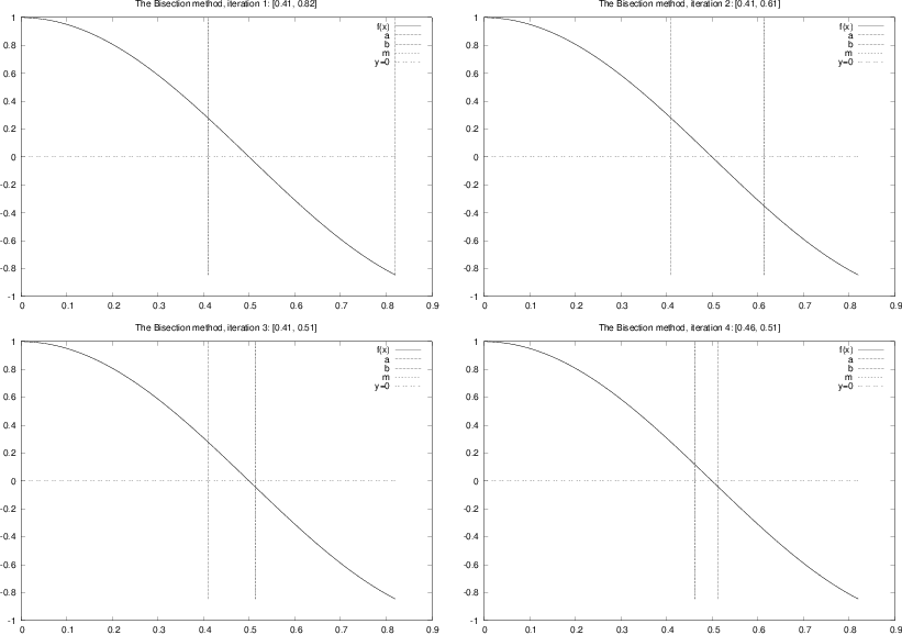
Figure 2 displays graphically the first four steps of this algorithm for solving the equation $ \cos (\pi x)=0 $, starting with the interval $ [0, 0.82] $. The graphs are automatically produced by the program bisection_movie.py, which was run as follows for this particular example:

bisection_movie.py 'cos(pi*x)' 0 0.82

The first command-line argument is the formula for $ f(x) $, the next is $ a $, and the final is $ b $.

Figure 2: Illustration of the first four iterations of the Bisection algorithm for solving $ \cos (\pi x) =0 $. The vertical lines correspond to the current value of $ a $ and $ b $.

In the algorithm listed above, we recompute $ f(a) $ in each if-test, but this is not necessary if $ a $ has not changed since the last $ f(a) $ computations. It is a good habit in numerical programming to avoid redundant work. On modern computers the Bisection algorithm normally runs so fast that we can afford to do more work than necessary. However, if $ f(x) $ is not a simple formula, but computed by comprehensive calculations in a program, the evaluation of $ f $ might take minutes or even hours, and reducing the number of evaluations in the Bisection algorithm is then very important. We will therefore introduce extra variables in the algorithm above to save an $ f(m) $ evaluation in each iteration in the for loop:

f_a = f(a)
for i in range(0, n+1):
    m = (a + b)/2
    f_m = f(m)
    if f_a*f_m <= 0:
        b = m   # root is in left half
    else:
        a = m   # root is in right half
        f_a = f_m

# f(x) has a root in [a,b]

To execute the algorithm above, we need to specify $ n $. Say we want to be sure that the root lies in an interval of maximum extent $ \epsilon $. After $ n $ iterations the length of our current interval is $ 2^{-n}(b-a) $, if $ [a,b] $ is the initial interval. The current interval is sufficiently small if $$ \begin{equation*} 2^{-n}(b-a) = \epsilon,\end{equation*} $$ which implies $$ \begin{equation} n = - {\ln\epsilon -\ln (b-a)\over\ln 2}\tp \tag{6} \end{equation} $$

Instead of calculating this $ n $, we may simply stop the iterations when the length of the current interval is less than $ \epsilon $. The loop is then naturally implemented as a while loop testing on whether $ b-a \leq\epsilon $. To make the algorithm more foolproof, we also insert a test to ensure that $ f(x) $ really changes sign in the initial interval. This guarantees a root in $ [a,b] $. (However, $ f(a)f(b) < 0 $ is not a necessary condition if there is an even number of roots in the initial interval.)

Our final version of the Bisection algorithm now becomes

f_a=f(a)
if f_a*f(b) > 0:
    # error: f does not change sign in [a,b]

i = 0
while b-a > epsilon:
    i = i + 1
    m = (a + b)/2
    f_m = f(m)
    if f_a*f_m <= 0:
        b = m  # root is in left half
    else:
        a = m  # root is in right half
        f_a = f_m

# if x is the real root, |x-m| < epsilon

This is the algorithm we aim to implement in a Python program.

A direct translation of the previous algorithm to a valid Python program is a matter of some minor edits:

eps = 1E-5
a, b = 0, 10

fa = f(a)
if fa*f(b) > 0:
    print 'f(x) does not change sign in [%g,%g].' % (a, b)
    sys.exit(1)

i = 0   # iteration counter
while b-a > eps:
    i += 1
    m = (a + b)/2.0
    fm = f(m)
    if fa*fm <= 0:
        b = m  # root is in left half of [a,b]
    else:
        a = m  # root is in right half of [a,b]
        fa = fm
    print 'Iteration %d: interval=[%g, %g]' % (i, a, b)
    
x = m          # this is the approximate root
print 'The root is', x, 'found in', i, 'iterations'
print 'f(%g)=%g' % (x, f(x))

This program is found in the file bisection_v1.py.

Verification

To verify the implementation in bisection_v1.py we choose a very simple $ f(x) $ where we know the exact root. One suitable example is a linear function, $ f(x)=2x-3 $ such that $ x=3/2 $ is the root of $ f $. As can be seen from the source code above, we have inserted a print statement inside the while loop to control that the program really does the right things. Running the program yields the output

Iteration 1: interval=[0, 5]
Iteration 2: interval=[0, 2.5]
Iteration 3: interval=[1.25, 2.5]
Iteration 4: interval=[1.25, 1.875]
...
Iteration 19: interval=[1.5, 1.50002]
Iteration 20: interval=[1.5, 1.50001]
The root is 1.50000572205 found in 20 iterations
f(1.50001)=1.14441e-05

It seems that the implementation works. Further checks should include hand calculations for the first (say) three iterations and comparison of the results with the program.

Making a function

The previous implementation of the bisection algorithm is fine for many purposes. To solve a new problem $ f(x)=0 $ it is just necessary to change the f(x) function in the program. However, if we encounter solving $ f(x)=0 $ in another program in another context, we must put the bisection algorithm into that program in the right place. This is simple in practice, but it requires some careful work, and it is easy to make errors. The task of solving $ f(x)=0 $ by the bisection algorithm is much simpler and safer if we have that algorithm available as a function in a module. Then we can just import the function and call it. This requires a minimum of writing in later programs.

When you have a "flat" program as shown above, without basic steps in the program collected in functions, you should always consider dividing the code into functions. The reason is that parts of the program will be much easier to reuse in other programs. You save coding, and that is a good rule! A program with functions is also easier to understand, because statements are collected into logical, separate units, which is another good rule! In a mathematical context, functions are particularly important since they naturally split the code into general algorithms (like the bisection algorithm) and a problem-specific part (like a special choice of $ f(x) $).

Shuffling statements in a program around to form a new and better designed version of the program is called refactoring. We shall now refactor the bisection_v1.py program by putting the statements in the bisection algorithm in a function bisection. This function naturally takes $ f(x) $, $ a $, $ b $, and $ \epsilon $ as parameters and returns the found root, perhaps together with the number of iterations required:

def bisection(f, a, b, eps):
    fa = f(a)
    if fa*f(b) > 0:
        return None, 0

    i = 0   # iteration counter
    while b-a > eps:
        i += 1
        m = (a + b)/2.0
        fm = f(m)
        if fa*fm <= 0:
            b = m  # root is in left half of [a,b]
        else:
            a = m  # root is in right half of [a,b]
            fa = fm
    return m, i

After this function we can have a test program:

def f(x):
    return 2*x - 3   # one root x=1.5

x, iter = bisection(f, a=0, b=10, eps=1E-5)
if x is None:
    print 'f(x) does not change sign in [%g,%g].' % (a, b)
else:
    print 'The root is', x, 'found in', iter, 'iterations'
    print 'f(%g)=%g' % (x, f(x))

The complete code is found in file bisection_v2.py.

Making a test function

Rather than having a main program as above for verifying the implementation, we should make a test function test_bisection as described in the section Verification of the module code. To this end, we move the statements above inside a function, drop the output, but instead make a boolean variable success that is True if the test is passed and False otherwise. Then we do assert success, msg, which will abort the program if the test fails. The msg variable is a string with more explanation of what went wrong the test fails. A test function with this structure is easy to integrate into the widely used testing frameworks nose and pytest, and there are no good reasons for not adopting this structure. The code checking that the root is within a distance $ \epsilon $ to the exact root becomes

def test_bisection():
    def f(x):
        return 2*x - 3   # one root x=1.5

    eps = 1E-5
    x_expected = 1.5
    x, iter = bisection(f, a=0, b=10, eps=eps)
    success = abs(x - x_expected) < eps  # test within eps tolerance
    assert success, 'found x=%g != 1.5' % x

Making a module

A motivating factor for implementing the bisection algorithm as a function bisection was that we could import this function in other programs to solve $ f(x)=0 $ equations. We therefore need to make a module file bisection.py such that we can do, e.g.,

from bisection import bisection
x, iter = bisection(lambda x: x**3 + 2*x -1, -10, 10, 1E-5)

A module file should not execute a main program, but just define functions, import modules, and define global variables. Any execution of a main program must take place in the test block, otherwise the import statement will start executing the main program, resulting in very disturbing statements for another program that wants to solve a different $ f(x)=0 $ equation.

The bisection_v2.py file had a main program that was just a simple test for checking that the bisection algorithm works for a linear function. We took this main program and wrapped in a test function test_bisection above. To run the test, we make the call to this function from the test block:

if __name__ == '__main__':
    test_bisection()

This is all that is demanded to turn the file bisection_v2.py into a proper module file bisection.py.

Defining a user interface

It is nice to have our bisection module do more than just test itself: there should be a user interface such that we can solve real problems $ f(x)=0 $, where $ f(x) $, $ a $, $ b $, and $ \epsilon $ are defined on the command line by the user. A dedicated function can read from the command line and return the data as Python object. For reading the function $ f(x) $ we can either apply eval on the command-line argument, or use the more sophisticated StringFunction tool from the section Turning string expressions into functions. With eval we need to import functions from the math module in case the user have such functions in the expression for $ f(x) $. With StringFunction this is not necessary.

A get_input() for getting input from the command line can be implemented as

def get_input():
    """Get f, a, b, eps from the command line."""
    from scitools.std import StringFunction
    try:
        f = StringFunction(sys.argv[1])
        a = float(sys.argv[2])
        b = float(sys.argv[3])
        eps = float(sys.argv[4])
    except IndexError:
        print 'Usage %s: f a b eps' % sys.argv[0]
        sys.exit(1)
    return f, a, b, eps

To solve the corresponding $ f(x)=0 $ problem, we simply add a branch in the if test in the test block:

if __name__ == '__main__':
    import sys
    if len(sys.argv) >= 2 and sys.argv[1] == 'test':
        test_bisection()
    else:
        f, a, b, eps = get_input()
        x, iter = bisection(f, a, b, eps)
        print 'Found root x=%g in %d iterations' % (x, iter)

Desired properties of a module. Our bisection.py code is a complete module file with the following generally desired features of Python modules:

other programs can import the bisection function,
the module can test itself (with a pytest/nose-compatible test function),
the module file can be run as a program with a user interface where a general rooting finding problem can be specified in terms of a formula for $ f(x) $ along with the parameters $ a $, $ b $, and $ \epsilon $.

Using the module

Suppose you want to solve $ x/(x-1)=\sin x $ using the bisection module. What do you have to do? First, you must reformulate the equation as $ f(x)=0 $, i.e., $ x/(x-1)-\sin x = 0 $, or maybe multiply by $ x-1 $ to get $ f(x)=x-(x-1)\sin x $.

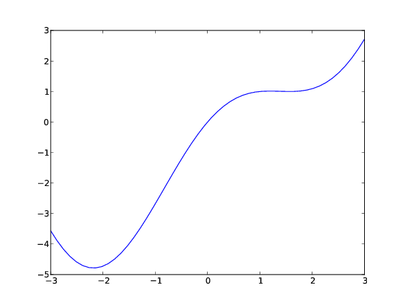
It is required to identify an interval for the root. By evaluating $ f(x) $ for some points $ x $ one can be trial and error locate an interval. A more convenient approach is to plot the function $ f(x) $ and visually inspect where a root is. We start ipython --pylab and write

In [1]: x = linspace(-3, 3, 50)  # generate 50 coordinates in [-3,3]

In [2]: y = x - (x-1)*sin(x)

In [3]: plot(x, y)

Figure 3 shows $ f(x) $ and we clearly see that, e.g., $ [-2, 1] $ is an appropriate interval.

Figure 3: Plot of $ f(x)=x - \sin (x) $.

The next step is to run the Bisection algorithm. There are two possibilities:

make a program where you code $ f(x) $ and run the bisection function, or
run the bisection.py program directly.

The latter approach is the simplest:

bisection.py "x - (x-1)*sin(x)" -2 1 1E-5
Found root x=-1.90735e-06 in 19 iterations

The alternative approach is to make a program:

from bisection import bisection
from math import sin

def f(x):
    return x - (x-1)*sin(x)

x, iter = bisection(f, a=-2, b=1, eps=1E-5)
print x, iter

Potential problems with the software

Let us solve

$ x = \tanh x $ with start interval $ [-10,10] $ and $ \epsilon=10^{-6} $,
$ x^5 = \tanh (x^5) $ with start interval $ [-10,10] $ and $ \epsilon=10^{-6} $.

Both equations have one root $ x=0 $.

bisection.py "x-tanh(x)" -10 10
Found root x=-5.96046e-07 in 25 iterations

bisection.py "x**5-tanh(x**5)" -10 10
Found root x=-0.0266892 in 25 iterations

These results look strange. In both cases we halve the start interval $ [-10,10] $ 25 times, but in the second case we end up with a much less accurate root although the value of $ \epsilon $ is the same. A closer inspection of what goes on in the bisection algorithm reveals that the inaccuracy is caused by rounding errors. As $ a, b, m\rightarrow 0 $, raising a small number to the fifth power in the expression for $ f(x) $ yields a much smaller result. Subtracting a very small number $ \tanh x^5 $ from another very small number $ x^5 $ may result in a small number with wrong sign, and the sign of $ f $ is essential in the bisection algorithm. We encourage the reader to graphically inspect this behavior by running these two examples with the bisection_plot.py program using a smaller interval $ [-1,1] $ to better see what is going on. The command-line arguments for the bisection_plot.py program are 'x-tanh(x)' -1 1 and 'x**5-tanh(x**5)' -1 1. The very flat area, in the latter case, where $ f(x)\approx 0 $ for $ x\in [-1/2, 1/2] $ illustrates well that it is difficult to locate an exact root.

Distributing the bisection module to others

The Python standard for installing software is to run a setup.py program,

Terminal> sudo python setup.py install

to install the system. The relevant setup.py for the bisection module arises from substituting the name interest by bisection in the setup.py file listed in the section Distributing modules. You can then distribute bisection.py and setup.py together.